Machine learning-driven decision support tools ought to assist users in detecting prospective advantages and risks. Widespread model-independent explanation frameworks can pinpoint elements underpinning specific forecasts—addressing queries like "What factors affect sales?" or "Why did sales decline?"—yet fail to indicate the actionable steps an individual can or should take to achieve a more favorable result. Although counterfactual explanation methods target actionable interventions and occasionally account for feasibility, they generally overlook viability for real-time systems like interactive question-answering platforms. In this study, we bridge this divide by proposing a unique model-agnostic technique that details concrete, viable adjustments capable of altering the predictions of a sophisticated Black Box AI framework for a specific instance; furthermore, we evaluate its practical utility by evaluating its computational speed in real time alongside its capacity to discover executable modifications. The developed approach leverages the target instance to produce high-precision explanations, subsequently employing a secondary mechanism to identify achievable minimally-contrastive counterfactual explanations (AMCC) by restricting the exploration space exclusively to modifications that adhere to domain-specific restrictions. Utilizing a well-established dataset, we assessed the classification procedure to determine both the success rate and the computational duration necessary to pinpoint valid counterfactual alternatives. Within the context of a classifier maintaining 90% accuracy, our proposed algorithm successfully extracted AMCC explanations in 47% of instances (38 of 81), requiring an average generation time of 80 ms. These outcomes confirm the efficiency of the algorithm in rapidly generating AMCC explanations, establishing its appropriateness for real-time deployments. The AMCC approach improves the interpretability of obscure Black Box AI models, thereby assisting stakeholders in analyzing corrective techniques or evaluating prospective consequences.
Explainable Artificial Intelligence (XAI) fulfills a variety of objectives, such as bolstering user confidence in an opaque Black Box architecture [1, 2] or improving the user's comprehension of how the model operates when encountering novel data instances [3]. An essential capability desired by users, which remains insufficiently realized in current XAI systems, involves resolving inquiries regarding actionable measures to modify a predicted forecast. This form of XAI is highly valuable for domains centered on behavioral modifications—such as mentoring, guidance, or coaching within healthcare, education, or personal finance—where the anticipated advantages of an intervention and its probability of success determine both the launch and long-term adherence to behavioral shifts [4-7].
Our primary focus centers on contexts wherein individuals formulate what are known as SMART goals. These SMART targets are characterized as specific, measurable, achievable, relevant, and time-bound [8, 9]. This mode of goal configuration would be enhanced by high-precision explanations, which specify the exact enabling value of a variable rather than merely identifying the feature name. (See Table 1 for some examples of high-precision explanations.) Additionally, we emphasize explanations that can be computed synchronously during an active dialogue, given that interactive engagement has been demonstrated to foster higher levels of trust in decision-enabling software compared to conventional web-centric graphical user interfaces [10].
Table 1. Examples of high-precision explanations generated for tabular data from [3].
Adult Income Classification Rules
|
|
Condition | Predicted Income Category |
No reported capital gain or capital loss, and marital status is never married | ≤ 50 K |
Country of residence is the US, marital status is married, and weekly working hours exceed 45 | > 50 K |
Loan Approval Assessment Rules |
|
Condition | Predicted Loan Outcome |
FICO score ≤ 649 | Bad loan |
649 ≤ FICO score ≤ 699 and 5,400 ≤ loan amount ≤ 10,000 | Good loan |
Explanatory descriptions that delineate scenarios leading to an alternate outcome relative to an observed case are termed counterfactuals. For many users, counterfactual structures represent the most intuitive and inherent style of explanation. In fact, foundational studies across cognitive psychology, philosophy, and the social sciences indicate that human expectations for "why" queries are best met by explanations that exhibit contrastive, selective, and socially interactive properties [11]—implying a strong preference for solution-oriented responses. The requirement for explanations that assist in correcting unfavorable predictions is further validated by contemporary user research in XAI, revealing that prompts aimed at optimizing an output rank among the top ten inquiry types users present to AI systems, alongside standard, broader "why" inquiries [12]. Wachter et al. [13] suggested that counterfactual and contrastive explanations (CCE) serve as a potent methodology for XAI, and recent comprehensive reviews highlight an escalating focus on CCE within the explainability research community [14].
When designing interventions, evaluating the feasibility of realizing a given counterfactual is crucial [15], meaning that the prescribed adjustment must be within the realm of a person's volitional actions. Isolating a sequence of viable actions represents a distinct subfield of counterfactual modeling designated as algorithmic recourse, which shares theoretical ties with causal machine learning paradigms [16, 17]. Attainability dictates that a domain-relevant action must exist that yields the intended alteration as a consequence, either via a direct mechanism—such as walking to alter a physical activity metric—or indirectly via transitioning a state of information. As an illustration, a clinician might request a diagnostic screening to confirm or dismiss a suspected medical condition.
In this work, we assume the availability of an underlying knowledge framework that supplies this contextual data, a premise that differentiates our strategy from frameworks attempting to deduce feasibility purely from observational datasets. Given that pathways to recourse are typically constrained, establishing such a domain model is straightforward, though it introduces certain practical considerations. For instance, when only a minimal subset of adjustments is viable, questions arise regarding the frequency with which recourse can be successfully established, the computational complexity involved in discovering appropriate pathways, and whether successful strategies can be produced rapidly enough to support immediate user engagement. Human-computer interaction literature suggests that the optimal response latency for conveying recourse options during keyboard-driven or mobile interactions should remain below 200 ms on desktop environments and under 500 ms for mobile platforms [18, 19].
We introduce a two-stage paradigm tailored to uncover realistic counterfactual alternatives suitable for real-time systems: the initial stage extracts high-precision explanations for the baseline prediction, followed by a subsequent stage that identifies actionable changes forecasted by the AI model to yield the target output. When successfully executed, this technique enables an architecture to handle both "why" and "what can be done" queries within a unified context. Formally, this mechanism generates explanations categorized as local, model-agnostic, high-precision, and achievable minimally-contrastive counterfactuals—notions that are formally delineated below.
Model-agnostic explanations characterize how an algorithm responds to diverse circumstances or inputs, rather than seeking to deconstruct its internal operational logic. Consequently, this methodology remains applicable across an array of machine learning architectures, including complex systems that fail to produce explicit rules or inherently support transparency [1].
Local explanations clarify the behavior of a predictive model for a specific data instance rather than summarizing its comprehensive global behavior. Within the tabular data contexts evaluated here, an individual instance consists of a collection of features, with each feature mapped to a value from a predefined set of permissible options, while the outcome represents a discrete class variable designated as the "target". Such local, model-independent explanations are typically uncovered by systematically perturbing feature attributes of the target test instance to isolate modifications that alter the objective prediction [1, 20].
High-precision explanations constitute local interpretations that specify both the relevant features and the precise values or numerical intervals required to sustain a given classification. For example, Anchors [3] represent high-precision local explanatory frameworks that isolate features capable of validating a specific output, regardless of the values assumed by remaining attributes.
Contrastive counterfactual explanations are local insights that attain an alternative target outcome T2 that is complementary to the baseline prediction T1 by modifying the values of a selected subset of input features for a given instance [21]. While these attributes may possess a causal linkage to the prediction, explicit causal structures are not strictly required to generate counterfactuals; an effective approximation can be derived by utilizing the optimized AI model to generate predictions for a contrastive instance [22].
Achievable contrastive counterfactual explanations represent local interpretations that realize an alternative target prediction T2 complementary to the baseline output T1 by strictly altering attributes that the subject of the decision-making platform can realistically modify. This data is highly dependent on the operational domain and specific application. We operate under the premise that all mutable features and their associated operational boundaries are supplied to the system, ensuring that attribute perturbations conform strictly to these guidelines. (In the case of socially interactive deployments, such as conversational interfaces, the architecture should also possess access to plain-language descriptions detailing the actions required to attain the targeted feature values).
Minimally-contrastive counterfactual explanations are local insights that reach an alternative objective T2 complementary to the original prediction T1 through a minimal collection of feature adjustments. Formally, if 𝑀𝐶𝐶𝑗 represents a minimally-contrastive explanation defined as 𝑀𝐶𝐶𝑗≡{𝑚1,𝑚2,…,𝑚𝑗}, then for any arbitrary component 𝑚𝑖∈𝑀𝐶𝐶𝑗, the reduced set 𝑀𝐶𝐶𝑗∖{𝑚𝑖} fails to yield T2. It is intuitively clear that users generally favor minimizing the total number of modifications, though individual priorities dictate preferences when choosing among distinct sets of changing features.
The research most intimately aligned with our proposed methodology is that of Poyiadzi et al. [23], who developed a framework for Feasible and Actionable Counterfactual Explanations (FACE). The FACE architecture relies on a modification of Dijkstra’s shortest path algorithm. This technique constructs a graph composed of data instances that are structurally comparable to a target test case. Within this graph structure, nodes represent individual instances, while edges connect pairs of instances that vary by the value of a single feature, provided that the corresponding adjustment is deemed actionable and practical for the target user according to a predefined condition function. Furthermore, FACE permits the integration of a "weight" function to represent user preferences regarding distinct categories of feature changes. Although this methodology yields local, model-agnostic counterfactual outcomes, it typically identifies only a isolated data point rather than a high-precision explanation, resembling most non-anchor-based strategies. Moreover, the authors omit details regarding the computational duration required to construct or traverse this graph structure for a given dataset under a restricted set of actionable attributes.
Preserving the agency of individuals over how machine learning models impact their personal lives serves as the core motivation behind "Actionable Recourse in Linear Classification" [24]. In their study, the authors introduce the concept of "recourse," which denotes the capacity of a human agent to alter a model's prediction by adjusting "actionable" input features. To accomplish this, they advocate for integer programming methodologies optimized for remediation within linear classification contexts; however, they do not evaluate real-time computational performance.
Another relevant strategy is presented by Mothilal et al. [25], who introduce an approach to isolate a diverse collection of feasible counterfactual actions by synthesizing a suite of distinct, viable counterexamples. Their framework produces novel contrastive instances while simultaneously evaluating a diversity metric across the synthesized cohort. Feasibility is determined using the proximity-based approach originally introduced by Wachter et al. [13], rather than relying on an explicit domain model. Similarly, Karimi et al. [15] propose an optimization-based technique designed to uncover a minimum-cost sequence of actions (modeled as structural interventions) that yield a counterfactual instance with the desired target prediction. Their approach associates costs directly with actions (edges) instead of features, acknowledging that different modifications to a single attribute may carry varying levels of acceptability. While the authors do not supply an explicit algorithmic formulation or implementation, they recommend utilizing the Abduction-Action-Prediction framework established by Pearl [22]. Consequently, the conditions under which this technique remains viable for real-time interactive systems remain unverified.
The primary intent of this study is to introduce a real-time, high-precision, model-agnostic approach to algorithmic recourse. The methodology involves adapting and expanding the capabilities of the local, model-agnostic explanation framework introduced in "Anchors: High-Precision Model-Agnostic Explanations" and evaluating its viability within interactive applications. The central modification involves leveraging this framework to extract minimally-contrastive counterfactuals by focusing exclusively on achievable, modifiable attributes that simultaneously serve as anchors.
Our investigation centers on two primary research questions: (1) when the feature space is restricted solely to plausibly actionable attributes, how frequently can the anchor-based strategy identify at least one explanation that functions as an effective intervention within a dataset tailored for algorithmic recourse? and (2) under these constraints, what is the computational speed with which such recourse can be identified? Secondary to these inquiries, we evaluate how performance is influenced by adjusting an internal parameter of the anchor algorithm—specifically the beam size—which regulates the volume of alternative candidates maintained under consideration during coverage maximization.
To identify counterfactual paths, our methodology investigates alternative states of the original instances by perturbing one feature at a time and evaluating the resulting output through the trained classifier. The principal aim of this process is to isolate a variation of a target instance that successfully shifts the classifier's baseline, suboptimal forecast into a more desirable target classification, while respecting domain constraints and user preferences.
Our emphasis on discovering achievable minimally-contrastive counterfactuals (AMCC) led us to utilize Breadth-First Search (BFS), a graph traversal technique that systematically examines all nodes at a given depth layer before moving deeper into the graph structure. We modified the traditional BFS framework to align with our specific objective, yielding a variant designated as "BFS-AMCC," which is outlined in Algorithm 1. In keeping with typical AI search heuristics, BFS-AMCC operates without a preconstructed graph; instead, it synthesizes nodes dynamically for each permissible category of feature adjustment. The algorithm can be configured to stop upon discovering a single successful counterfactual that requires the minimum number of feature modifications, or it can be permitted to continue searching until it either exhausts the search space or satisfies a predefined termination criterion.
The execution of BFS-AMCC begins by inserting the baseline instance into a processing queue. In the primary execution loop, an instance is removed from the queue to undergo model prediction. If the prediction for this modified instance diverges from the baseline output, it is categorized as a successful modification and the execution terminates. Otherwise, the algorithm identifies features that are eligible for potential adjustment. In scenarios where explicit feature indices are not provided, the framework treats all categorical feature dimensions as modifiable.
Furthermore, BFS-AMCC accommodates an optional collection of "transitionrules" assigned to the features. These parameters define permissible transitions between distinct feature states, ensuring the algorithm restricts its search to realistic and achievable modifications of the source data. When a "transitionrule" is enforced for a specific feature, the algorithm accepts the modified feature value only if the evaluation function returns true when comparing the current state with the prospective state. These transition rules are inherently domain-specific and ideally derived from an ontology, though they can be encoded directly for simpler data structures.
Throughout its iterative execution, BFS-AMCC evaluates each feature index sequentially, generating a modified instance for every valid feature value perturbation and placing it into the queue. This cyclical process continues until a perturbed instance successfully triggers a shift from the baseline prediction to the intended target outcome, or until the processing queue becomes empty.
Ultimately, BFS-AMCC outputs the successfully modified data point—representing an achievable, minimally-contrastive counterfactual that steers the classifier’s baseline prediction toward a preferred target class. If no valid modification is identified, the procedure outputs "None". This systematic approach guarantees the identification of a locally-minimal counterfactual, providing enhanced interpretability owing to its minimal feature divergence from the source instance.
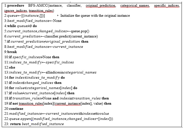
Algorithm 1. BFS for achievable minimally-contrastive counterfactuals to change the predicted value
The empirical assessment method utilized in this study is detailed in Algorithm 2 and is structured to analyze the capabilities of our counterfactual generation framework, specifically BFS-AMCC. The primary goals are to determine the percentage of successfully generated counterfactual cases and to quantify the execution duration required for each successful instance. These resulting metrics are compiled within a Python dictionary for subsequent investigation.
To enhance the computational efficiency and operational feasibility of this methodology, an execution threshold of 5 s per instance is enforced utilizing the 'signal' module in Python. This temporal constraint serves to eliminate extreme statistical outliers while preserving an appropriate equilibrium between rigorous exploration and processing duration. Furthermore, this threshold is highly conservative, considering that the baseline for real-time user engagement typically spans from 200 to 500 ms [18, 19]. In practical applications, this execution ceiling is rarely encountered, occurring almost exclusively when no viable recourse path exists.
The procedure begins by initializing tracking variables for both successful and unsuccessful instances, alongside a timer dedicated to monitoring the processing duration of each distinct case.
The primary execution loop of the assessment framework iterates through each entry within the provided 'suboptimalinstances' array, which contains the cases identified as candidates for correction. For every individual instance, the system extracts both the actual ground-truth label and the corresponding prediction generated by the classifier.
When the prediction from the classifier aligns with the actual ground-truth value, the system deploys the 'AnchorTabularExplainer' to pinpoint high-precision features. These identified characteristics are subsequently integrated into the BFS-AMCC workflow to steer the creation of adjusted instances.
Following this, the system executes the BFS-AMCC function (Algorithm 1) to construct an altered instance within the designated temporal limit. If a valid modified instance is produced before the timeout, the system increments the success counter, logs the elapsed duration, and records the specific modifications. Conversely, if an acceptable counterfactual cannot be established within the allocated timeframe, a 'TimeoutError' is triggered, prompting the system to transition to the subsequent instance while incrementing the failure tracker.
Once all cases within the 'suboptimalinstances' array have been evaluated, the procedure outputs the 'metrics' dictionary. This data structure offers an exhaustive overview of the framework's effectiveness, encompassing the total counts of successful and failed cases, the aggregate processing duration, and a comprehensive registry of alterations for every successful counterfactual instance.
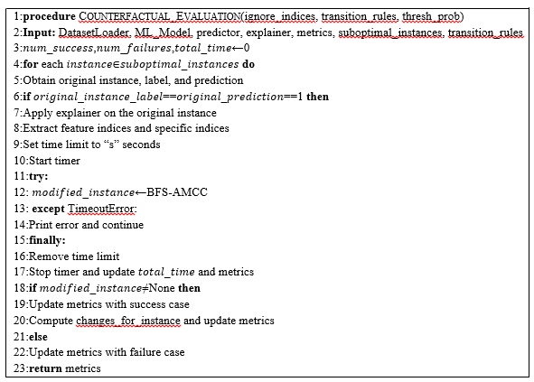
Algorithm 2. Evaluation of Counterfactual Generation
This section outlines each phase of our experimental evaluation alongside the corresponding outcomes. The assessment measures the computational difficulty of discovering an AMCC explanation—quantified by both the success rate and execution time—utilizing a representative dataset. Additionally, we conduct preliminary tests to construct an idealized classifier, followed by investigations where a critical variable within the Anchors framework, the 'beam size', is systematically adjusted. Finally, we showcase specific instances of the AMCC explanations generated for a selection of test cases, including their respective processing durations.
We utilized a publicly accessible tabular dataset, HMEQ, which contains multiple actionable attributes. The HMEQ dataset originates from the mortgage lending sector, where the predicted target variables are defined as {GOOD, BAD}. In this context, a bad loan denotes a case that culminated in a default or a significant repayment delinquency, whereas a good loan signifies a debt that was fulfilled according to schedule. This dataset was sourced from Kaggle.
The dataset comprises a total of 5960 records representing individual home equity loan accounts, wherein the unfavorable classification, f=1 (BAD), is present in approximately 20% of the observations (n = 1189). For each loan applicant, 12 distinct input variables were captured; among these, we identified seven variables as actionable, which are detailed in Table 2 along with their corresponding recourse paths.
We identified multiple instances where attribute modifications would realistically be practical or attainable in only a single direction; consequently, the features MORTDUE, DELINQ, NINCQ, and DEBTINC are constrained such that they can only be decreased, not increased.
Table 2. Actionable features in the HMEQ dataset including recourse actions.
Attribute | Description | Illustrative Recourse Strategy |
LOAN | Requested loan amount submitted by the applicant | Increase or decrease the requested loan value |
MORTDUE | Outstanding balance remaining on the current mortgage | Reduce the mortgage balance through additional payments |
VALUE | Estimated market value of the property | Obtain a new property valuation or appraisal |
DELINQ | Count of delinquent credit accounts | Clear overdue credit obligations |
NINQ | Number of recent credit inquiries | Limit or postpone new credit applications |
CLNO | Total count of active credit lines | Open additional credit lines or close existing ones |
DEBTINC | Applicant’s debt-to-income (DTI) ratio | Lower overall debt by paying off a portion of outstanding liabilities |
It is worth noting that the majority of attributes within the HMEQ dataset consist of continuous numerical observations (e.g., total loan amounts, duration of employment, etc.). In order to optimize the efficacy of the linear architectures under evaluation, we initially partitioned these continuous variables into four broad categorical intervals using the KBinDiscretizer tool from sklearn.
Following data preparation, we analyzed the complexity of the underlying classification problem by utilizing the dataset to train two frequently deployed classification algorithms, measuring their performance through standard diagnostic criteria (Precision, Recall, and F1).
In this phase of the study, we compared the capabilities of Random Forest and XGBoost classification models. The Random Forest algorithm constructs an ensemble of independent decision trees during the training phase, utilizing randomized subsets of input features and data instances to minimize overfitting and boost the model's capacity for generalization. Conversely, XGBoost utilizes an iterative gradient-boosting methodology, sequentially engineering weak learners that explicitly correct the predictive errors committed by preceding models, thereby minimizing model bias and enhancing overall accuracy [26].
The deployment of these algorithms, as well as the procedure for synthesizing distinct feature permutations, was carried out using Python paired with the NumPy library to facilitate rapid mathematical processing. Furthermore, we leveraged Python's core processing capabilities during the post-processing phase to construct contrastive anchors, analyze shifts in predictive outcomes, and eliminate redundant supersets.
We commenced our quantitative investigation using two distinct machine learning models: Random Forest and XGBoost. The predictive capabilities of these models were measured via accuracy, precision, recall, and F1 score, evaluated across three distinct training-validation-testing data partitions: 80%-10%-10%, 70%-15%-15%, and 60%-20%-20%, as documented in Table 3.
Table 3. Performance metrics of Random Forest and XGBoost under different data split ratios.
Model | Data Split Ratio | F1 Score | Recall | Precision | Accuracy |
Random Forest | 80%-10%-10% | 0.75 | 0.63 | 0.92 | 0.90 |
70%-15%-15% | 0.71 | 0.58 | 0.92 | 0.90 | |
60%-20%-20% | 0.72 | 0.61 | 0.88 | 0.91 | |
XGBoost | 80%-10%-10% | 0.73 | 0.61 | 0.90 | 0.90 |
70%-15%-15% | 0.69 | 0.57 | 0.88 | 0.89 | |
60%-20%-20% | 0.72 | 0.62 | 0.85 | 0.91 |
The F1 metric for the XGBoost architecture displayed a stable trend across the majority of data configurations, experiencing a slight reduction specifically at the 70%-15%-15% split. On the other hand, the Random Forest model demonstrated a steady rise in its F1 metric as the share of training data expanded, peaking at a maximum value of 0.75 when paired with the 80%-10%-10% data partition.
Because the optimal F1 performance was produced by the Random Forest classifier configured with an 80%-10%-10% distribution, this specific model configuration and data split were selected for all subsequent counterfactual optimization testing.
Table 4 details the explicit hyperparameters designated for both the Random Forest and XGBoost architectures throughout these trials. These hyperparameter configurations were determined via empirical testing to maximize model performance on the training partitions, informed by our initial baseline tests with the dataset. For the Random Forest framework, we utilized the 'logloss' splitting criterion alongside log2 max features, incorporating 100 estimators and five concurrent jobs. In a similar fashion, the XGBoost framework was established with a 'logloss' evaluation metric, paired with targeted adjustments for tree depth, column subsampling by tree, and total estimator count.
Table 4. Parameters for Random Forest and XGBoost models.
Model | Configuration Parameters |
Random Forest | Number of trees (n_estimators) = 100; parallel processing jobs (n_jobs) = 5; splitting criterion = 'log_loss'; feature selection strategy (max_features) = 'log2' |
XGBoost | Evaluation metric (eval_metric) = 'logloss'; maximum tree depth (max_depth) = 6; subsampling ratio (subsample) = 0.8; column sampling per tree (colsample_bytree) = 0.8; number of boosting rounds/estimators (n_estimators) = 100 |
Following the selection of the primary machine learning architecture, the BFS-AMCC framework was systematically implemented on data instances that the model originally designated as ‘BAD’. Within this analytical phase, feature indices 4, 5, 6, 7, and 9—which represent REASON, JOB, YOJ, DEROG, and CLAGE, respectively—were established as immutable parameters. Furthermore, specific directional boundaries were enforced to block any positive value increases for four variables: DEBTINC, NINQ, DELINQ, and MORTDUE. This process isolated a subset of 81 instances from the test partition.
The empirical data tracking the success rate of BFS-AMCC revealed that, despite these rigorous operational constraints on attribute actionability, the system discovered viable adaptations for 38 out of the 81 cases, representing a success rate of 47%. Conversely, the algorithm failed to produce a valid counterfactual within the designated runtime limit for 43 instances. For this specific calculation, the top two extreme outliers were omitted due to an atypical processing duration of 2.75 s, an execution time roughly ten times greater than the observed average. These outcomes, illustrated in Figure 1, demonstrate the capability of the BFS-AMCC algorithm to identify effective and realistic modifications under restrictive conditions governed by fixed attributes and directional transition boundaries.
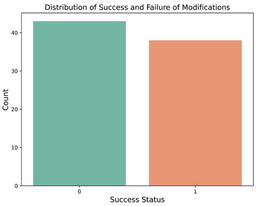
Figure 1. Distribution of success (1) and failure (0) of modifications.
To evaluate the operational readiness of the system for real-time applications, the processing intervals required for generation were recorded and organized into a histogram. Figure 2 illustrates the proportional distribution of the execution time for individual adjustments, revealing that over 90% of the modifications were resolved within 400 ms or less, irrespective of whether the generation was successful.
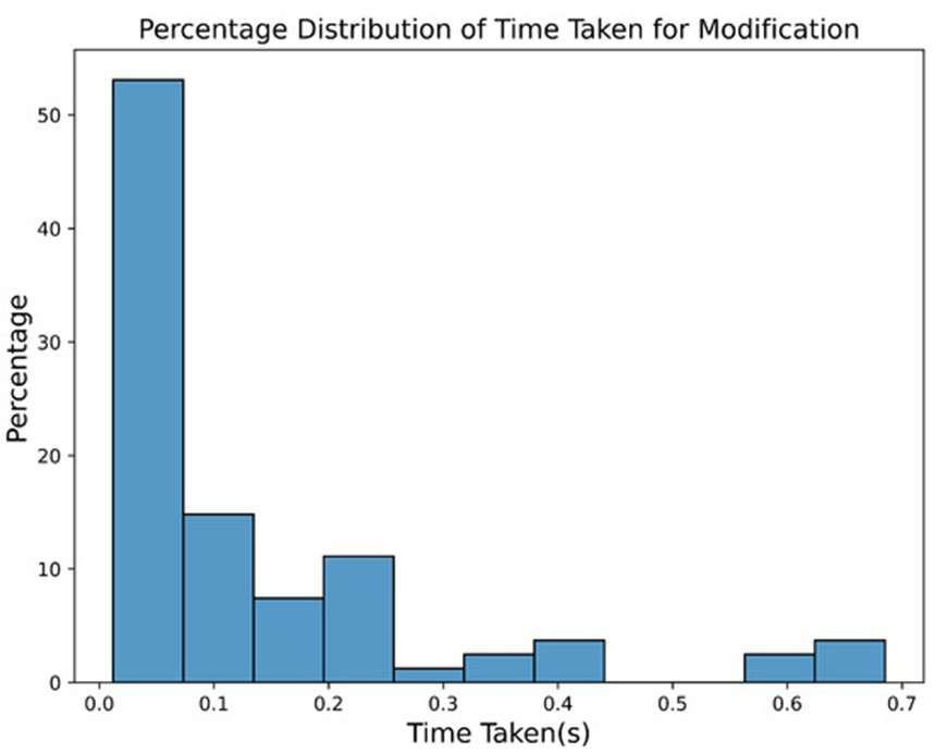
Figure 2. Distribution of time taken (in seconds) for modification.
Additionally, a comparative analysis of the execution durations between successful and failed modifications was conducted using a box plot, as displayed in Figure 3. The graphical distribution demonstrates that the median processing duration required to return an output remained substantially below 200 ms for both successful and unsuccessful attempts. This performance successfully satisfies the historically established latency thresholds required for interactive processing on diverse hardware platforms [18, 19]. This comparison validates the computational efficiency of the BFS-AMCC framework for integration into real-time interactive systems.
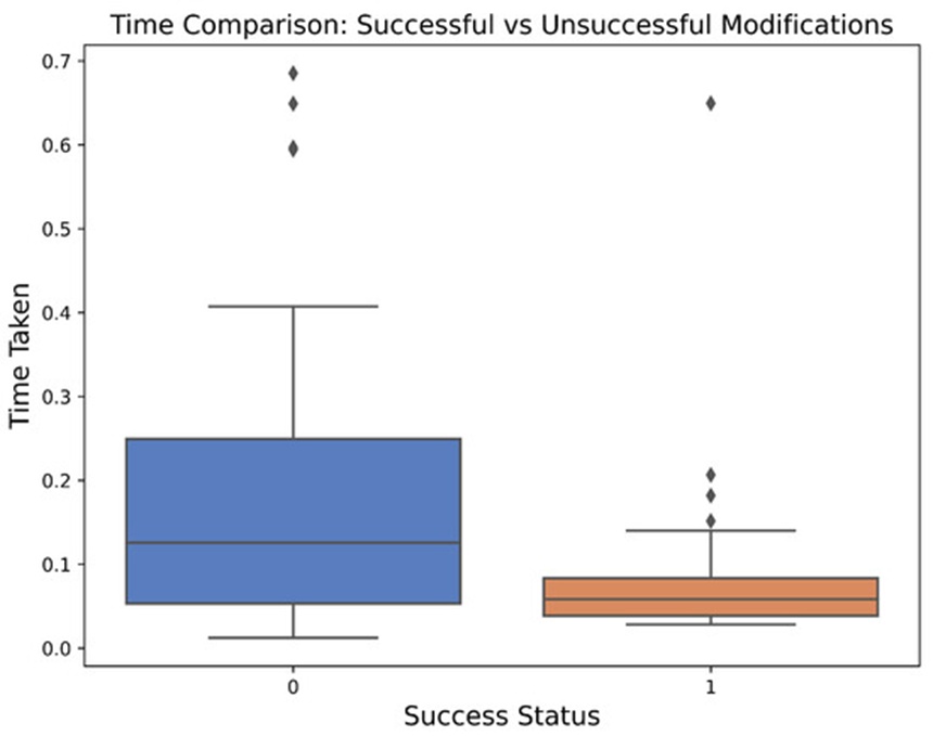
Figure 3. Comparison of time taken for successful (1) vs. unsuccessful (0) modifications.
Operating the Anchors framework requires the configuration of the 'beam size' hyperparameter, which dictates the maximum volume of candidate hypotheses retained during the state-space search, where candidates are ranked based on their data coverage properties. From a computational speed perspective, a restricted beam capacity might appear advantageous; however, an overly narrow beam can cause the premature elimination of viable candidates, thereby extending the total search trajectory. Because determining the ideal beam size is dependent on dataset characteristics and the number of mutable features, we analyzed a spectrum of beam values across two distinct operational environments: restricting BFS-AMCC to actionable features and directional rules (Ignore indices are TRUE) versus allowing full exploratory freedom (Ignore indices are False).
Table 5 summarizes the operational performance of the BFS-AMCC framework under three distinct beam dimensions, comparing the scenario involving ignored indices and transition rules (the standard deployment case) against unrestricted search flexibility. The metric for total time represents the cumulative processing duration across the entire test set (the mean values for individual cases are examined below). Unsurprisingly, the results indicate that permitting the framework complete latitude in feature adaptation—by configuring both ignored indices and transition boundaries to FALSE—improved the success metrics across all evaluated beam sizes. Nevertheless, this unconstrained state-space exploration introduced a substantial computational burden, as demonstrated by a significant elevation in overall execution time.
In contrast, applying domain constraints through ignored indices and transition rules (the TRUE operational state) led to a diminished success rate but achieved a substantial reduction in processing time. These findings highlight the necessity of precise hyperparameter calibration regarding beam size, alongside the introduction of pragmatic constraints on feature adjustments when optimizing the BFS-AMCC workflow. Consequently, a distinct trade-off exists between generation success, algorithmic efficiency, and the scale of permitted feature adjustments, which must be carefully balanced for each individual application domain.
Table 5. Performance metrics for different beam sizes and ignore indices conditions.
Ignore Indices | Total Time (s) | Failure | Success | Beam Size |
TRUE | 13.99 | 46 | 35 | 3 |
10.87 | 44 | 37 | 5 | |
11.39 | 43 | 38 | 10 | |
FALSE | 213.78 | 26 | 55 | 3 |
110.81 | 22 | 59 | 5 | |
151.1 | 22 | 59 | 10 |
Table 6 details the calculated average execution times broken down by successful and unsuccessful adjustments. The data show that the mean duration for a successful modification is merely 80 ms, which is significantly faster than the average duration of 190 ms recorded for failed generation attempts.
Table 6. Mean time for successful and unsuccessful modifications.
Success Status | Mean Time (s) |
Successful | 0.08 |
Unsuccessful | 0.19 |
As a definitive validation of the practical utility of the BFS-AMCC framework, we reviewed the specific actionable recommendations generated, as well as the time required to compute these explanations, for a selected sample of test cases. Figure 4 displays a series of representative instances detailing the feature adjustments alongside their respective computation times. All documented variations in feature values were performed by the BFS-AMCC framework on records that the classification model initially flagged as ‘BAD’. Each horizontal row details a single case, showing the adjusted variable values and the corresponding processing latency.
For instance, the fourth row displays a modification in the ‘DELINQ’ attribute from 4.0 to 2.0, which matches a reduction in delinquent lines of credit from the 11–15 category down to the 4–7 range. The time required to obtain this solution was 63 ms. As demonstrated by the compiled records, the processing duration consistently remained under 500 ms, even in scenarios where multiple features were adjusted concurrently. These observations illustrate the capability of the BFS-AMCC algorithm to optimize data records while maintaining a low computational overhead.
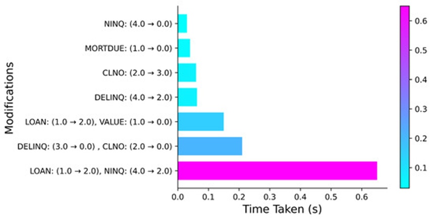
Figure 4. Variable modifications and their respective durations.
Broadly, the gathered evidence indicates that the BFS-AMCC framework can be successfully deployed to deliver high-precision explanations that adhere to predefined operational boundaries, including the classification of actionable attributes and permissible transition pathways. The success metrics for discovering achievable minimally-contrastive counterfactual explanations were found to be on par with those for unconstrained high-precision predictions, while requiring significantly lower processing latency. Across all evaluated beam configurations, the AMCC framework completed its execution in approximately one-tenth of the time demanded by an unconstrained search, consistently requiring less than 200 ms. The algorithm generated valid AMCC explanations in 47% of the evaluated scenarios (38 out of 81 test instances), with an average execution duration of merely 80 ms for successful cases. Consequently, our primary research questions have been successfully resolved.
Implementing this algorithm on an empirical, real-world lending dataset and verifying its capability to modify a substantial portion of records labeled as ‘BAD’ emphasizes the practical utility of BFS-AMCC. For instance, both organizational decision-makers and loan applicants can leverage this framework to pinpoint the necessary behavioral or financial modifications required to secure favorable outcomes, or alternatively, to recognize when no realistic path to recourse is available. Moreover, these analytical insights could offer valuable support for educational programs designed to elevate financial literacy.
As demonstrated by the proportional split between successful and failed alterations shown in Figure 1, the BFS-AMCC architecture successfully modifies the majority of evaluated instances, thereby answering our initial research inquiry regarding the capacity of the model to identify viable recourse. Furthermore, these algorithmic transformations are computed rapidly, generally within a 200 ms window, which resolves our second research question regarding the temporal efficiency of recourse identification. By embedding strict timeout parameters directly within the BFS-AMCC framework, the operational efficiency of the system in real-time environments can be optimized even further.
The experimental outcomes detailed in Table 5 demonstrate how the performance of the BFS-AMCC framework is driven by changes in the beam size and the status of the ignore-indices parameters. These patterns indicate that a careful balance between available computational resources and algorithmic throughput must be established and verified empirically. When the ignore indices parameter was set to TRUE, stable success rates were observed across different beam configurations, with narrower beam choices yielding greater processing efficiency. In contrast, configuring the ignore indices parameter to FALSE meant that increasing the beam size resulted in only a marginal gain in the success rate while introducing a substantial spike in computational latency. This finding highlights the critical need to carefully calibrate beam dimensions and configure ignore indices, a determination that is further validated by the necessity of omitting extreme outliers when the ignore indices parameter was set to FALSE.
The variance in execution duration between successful and unsuccessful instance modifications (as seen in Figure 3 and Table 6) highlights another fundamental characteristic of the system. While potentially counterintuitive at first glance, the accelerated processing of successful modifications is directly attributable to the breadth-first search mechanics of the BFS-AMCC algorithm, which inherently uncovers viable adjustments during the initial stages of state-space traversal. Conversely, failed modification attempts require an exhaustive exploration of the entire search space before the algorithm can definitively conclude that no valid counterfactual exists. This operational reality indicates that in production environments, it is entirely practical to implement a strict maximum execution time and return a negative outcome if that threshold is crossed.
Figure 4 illustrates the high efficiency of the BFS-AMCC framework when modifying data records. The capacity of the algorithm to alter multiple independent features simultaneously while maintaining low execution latencies demonstrates its optimized search and transformation mechanics. This performance underscores the scalability of the architecture and its appropriateness for complex deployment environments. Additionally, the successful generation of modifications under rigid constraints, such as the presence of entirely fixed variables, highlights its adaptability and functional versatility, thereby extending its prospective utility across a wide range of analytical problem domains.
Lastly, the superior performance exhibited by the Random Forest classifier in these trials emphasizes that model selection plays a pivotal role in this type of counterfactual analysis. This specific classifier's capacity to effectively navigate high-dimensional feature spaces and complex decision boundaries within the dataset likely explains its strong performance. This study provides useful insights into the functional interplay between different machine learning models and the BFS-AMCC pipeline, establishing a benchmark for future exploration. For instance, when dealing with datasets that feature a massive array of input variables, incorporating automated feature selection techniques represents a promising avenue for study.
Despite its demonstrated advantages, the BFS-AMCC methodology possesses several limitations that require acknowledgment. While the framework accommodates the enforcement of fixed variables via the ‘ignore indices’ parameter, isolating which specific attributes are truly actionable and determining their valid ranges of modification can be difficult in practical settings, frequently requiring deep domain-specific knowledge. Furthermore, defining an optimal execution timeout, particularly for scenarios where no realistic recourse path can be established, remains an open area for future investigation. Additionally, more comprehensive evaluations across a broader range of hyperparameter configurations are necessary to fully guarantee the robustness of the underlying machine learning models.
A detailed inspection of the HMEQ dataset reveals that the definition of achievability must be fundamentally connected to individual behaviors and asset transitions, structured in strict compliance with domain-specific limitations. For example, it is economically realistic for an individual to reduce their outstanding mortgage balance via accelerated principal payments; conversely, it is not realistic to instantly increase it. If a predictive model implies that a higher mortgage balance leads to a more favorable credit classification, it merely reflects the structural privileges associated with greater initial wealth. Within our framework, this domain complexity is controlled by applying targeted transition boundaries, such as explicitly restricting any upward adjustments to the ‘MORTDUE’ variable.
However, as illustrated in Figure 4, some of the permitted modifications may still require direct intervention or verification by the user. A clear example of this is the modification of the CLNO feature (2 → 3), which represents an increase in open credit accounts from the 18–35 interval up to the 36–53 range. The real-world feasibility of such a modification depends heavily on the user's unique financial situation and potential unmodeled dependencies between variables.
It is also critical to recognize that while certain modifications may accurately comply with the mathematical relationships embedded in the dataset and serve as valid baseline recommendations, their real-world practicality can vary widely based on an individual's unique situation. For example, the DELINQ modification (4.0 → 2.0) instructs the user to reduce the number of delinquent credit lines from a peak of 15 down to fewer than seven. The feasibility of achieving this outcome is intrinsically linked to external factors, such as the total volume of outstanding debt. Implementing an interactive deployment model would allow users to flag impractical recommendations, instructing the AMCC framework to dynamically redefine variables like DELINQ as immutable parameters. This interactive flexibility also supports targeted, "what-about-X" scenarios by rendering only feature X mutable during the search. Future iterations of this work could explore modifying the AMCC framework to use a dedicated beam search rather than a standard breadth-first search, thereby generating a broader portfolio of counterfactual options. These alternative pathways could then be ordered based on individual preferences or estimated probabilities of successful adoption. This strategy matches existing counterfactual research that advocates for presenting users with a diverse selection of interpretable options to ensure a comprehensive understanding.
The methodology proposed in this work successfully achieves the goal of identifying realistic, minimal counterfactuals without requiring the calculation of complex optimization metrics. Similar to the FACE framework introduced by Poyiadzi et al. [23], our algorithm integrates feasibility and actionability constraints in an entirely model-agnostic manner. However, unlike FACE, the AMCC workflow does not establish feasibility based on the density of observations within the training data, nor does it calculate data similarity metrics.
While both FACE and AMCC leverage path-search strategies to isolate counterfactual configurations—utilizing Dijkstra’s algorithm and breadth-first search, respectively, to map the shortest path—their underlying structures differ. BFS relies on a basic queue data structure, whereas Dijkstra’s algorithm utilizes weighted edges in tandem with a priority queue. Notably, the framework introduced here does not require the pre-construction of an explicit graph network before launching the search query. Instead, it systematically modifies instances on a feature-by-feature basis, implicitly generating a new node with each step to represent a minimal variation of its parent state. Furthermore, our empirical assessment integrates practical efficiency indicators, such as the exact processing duration required for counterfactual discovery, which is a dimension that has been largely overlooked in earlier literature.
In a similar vein to Poyiadzi et al., Mothilal et al. [25] frame the generation of minimal, achievable counterfactuals as a mathematical optimization challenge, which consequently demands continuous proximity and diversity computations. Their assessment criteria focus on F1-score, Recall, and Precision across multiple distinct datasets, though they omit temporal performance measures. Across the various datasets and techniques evaluated in their research, their framework recorded F1-scores spanning from 0.2 to 0.6, a performance tier that aligns closely with the 47% average success rate achieved by the AMCC framework in this study.
Subsequent investigations could systematically examine the precise impact of diverse underlying predictive architectures on the operational throughput of the BFS-AMCC pipeline. Additional work is needed to explore its adaptability when applied to datasets characterized by varying levels of feature volatility, and to assess alternative counterfactual generation strategies that might yield equivalent or superior performance. A compelling direction for future study involves extracting the domain-specific logic required by the algorithm from more comprehensive, generalized data structures, such as knowledge graphs [27]. Such developments would expand the deployment of AMCC within conversational AI agents engineered to foster long-term behavioral changes, such as optimized time management practices or increased physical activity [28, 29]. This prospective focus matches the trajectory of our current research initiatives.
Despite the structural complexities involved, the findings detailed in this study represent a crucial step forward in understanding and applying counterfactual explanations to improve the interpretability of machine learning models in both predictive and interventional contexts, establishing a firm baseline for future breakthroughs.
This paper introduces the BFS-AMCC algorithm as a dependable framework for identifying achievable, minimally-contrastive counterfactual explanations that can be seamlessly integrated with any machine learning model trained on tabular data. Delivering high-precision, model-agnostic counterfactual insights is crucial for modern automated decision-support networks, driving a paradigm shift from passive classification toward actionable intervention. In interactive deployments, when a user is faced with an unfavorable classification, they require clear explanations regarding the underlying causes along with practical strategies to secure a favorable decision.
Ideally, a production system should output these actionable insights within a processing latency of 200 to 500 ms, a threshold established as acceptable by prior human-computer interaction research. Significantly, this approach eliminates any dependency on complex mathematical metrics to evaluate feasibility. Instead, it leverages direct guidance from domain specialists to map permissible actions, while the underlying framework compiles valid alternatives within a fixed processing window. Any latent causal inconsistencies or contradictory variables are resolved through direct user collaboration, resulting in a finely tuned AMCC explanation. Consequently, this explainable AI framework remains transparent and highly interpretable for a diverse range of stakeholders. The real-time processing efficiency of this AMCC methodology highlights its viability for driving conversational systems built to guide users toward better outcomes.
In conclusion, the empirical findings compiled in this study validate that our BFS-AMCC framework routinely identifies at least one actionable explanation capable of guiding meaningful user intervention, all within an acceptable processing timeframe. This investigation therefore provides strong evidence supporting the overall efficacy of the BFS-AMCC framework. Furthermore, this approach fulfills essential operational requirements for real-world deployment and end-user comprehension, highlighting its practical value.
The following abbreviations are used in this manuscript:
AMCC | Achievable Minimally-Contrastive Counterfactual Explanation |
AI | Artificial Intelligence |
BFS | Breadth-First Search |
CCE | Contrastive Counterfactual Explanation |
RF | Random Forest |
XAI | Explainable Artificial Intelligence |
The authors thank their families for their continued patience and support.
None
The authors acknowledge the support of the Office of Dean of the College of Engineering & Applied Science at the University of Wisconsin-Milwaukee.
None
Open Access The author(s) retain copyright. This article is licensed under the Creative Commons Attribution-NonCommercial-ShareAlike 4.0 International License. It may be shared and adapted for non-commercial purposes with appropriate attribution, an indication of changes, and distribution of adaptations under the same license. Third-party material may be subject to separate terms identified in its credit line. View the license at https://creativecommons.org/licenses/by-nc-sa/4.0/.
 Transparent Intelligence Publishing