Artificial neural networks (ANNs) have frequently been deployed for classification objectives within functional magnetic resonance imaging (fMRI) research, though such analyses traditionally isolate only specific regional sub-volumes of the brain. Recent methodology has integrated shallow neural networks (SNNs) with explainable artificial intelligence (xAI) frameworks to uncover underlying mechanisms of neural processing. Although prior research validated this paradigm utilizing fMRI data from motor execution tasks, the current investigation implements this framework on Theory of Mind (ToM) cognitive tasks, leveraging data extracted from the Human Connectome Project (HCP) Young Adult repository. Cognitive paradigms introduce greater computational complexity due to the fundamentally non-linear dynamics of neural functions. The HCP multimodal parcellation brain atlas is utilized to partition the cortex, thereby guiding the systematic training, pruning, and subsequent retraining of an SNN. Shapley values are subsequently computed to decode the retrained architecture, with the resulting outputs benchmarked against a General Linear Model (GLM) analysis for empirical validation. The baseline network demonstrated a classification accuracy of 88.2%, which decreased to 80.0% following network pruning, and subsequently recovered to 84.7% after the retraining phase. The SHAP-derived explanations demonstrated strong convergence with both GLM observations and established neuroanatomical regions associated with ToM. This fMRI investigation effectively navigated a highly complex cognitive paradigm, illustrating the efficacy of explainability techniques in deciphering non-linear neurological dynamics. These outcomes indicate that xAI platforms, particularly knowledge extraction frameworks, offer substantial utility for progressing mental health research and neural state decoding applications.
When rigorously trained and supplied with sufficiently generalizable input data, artificial neural networks (ANNs) possess the capacity to distill critical insights from complex datasets, yielding models with robust predictive fidelity [1]. Functional magnetic resonance imaging (fMRI) serves as a foundational neuroimaging modality that generates four-dimensional (4D) representations of the active brain, supporting applications that extend from clinical psychiatry to neural decoding paradigms designed to map human cognition. While foundational attempts to implement ANNs for the interpretation of 4D fMRI data have been documented [2, 3], distinct methodological hurdles have historically limited the broader translation of these techniques for societal benefit. A comprehensive review of various machine learning algorithms applied to fMRI classification highlighted prominent reservations regarding the use of ANNs for these investigations [4]. These primary concerns encompass (1) whether the marginal gains in classification performance sufficiently offset the heightened structural complexity of ANN architectures; and (2) the inherent "black box" operational profile of these networks, which impedes straightforward explanation and interpretation. More recently, these specific methodological barriers have been directly addressed through frameworks engineered around the unique characteristics of fMRI data, producing outputs and models corroborating established neuroscientific paradigms [5, 6]. These developed pipelines, however, were restricted to motor execution paradigms and isolated within the motor cortex, where structure-function relationships are highly direct. The present investigation expands this methodology into the cognitive domain, seeking to generate models that demonstrate robust validation accuracy. Explainable artificial intelligence (xAI) techniques are integrated into the modeling pipeline to enhance transparency, explainability, and interpretability, thereby facilitating knowledge extraction [7, 8] and supporting the eventual realization of digital twin architectures of the cognitively active brain. The identified cortical regions are evaluated against established neuroanatomical literature for validation.
The collaborative potential of pairing artificial intelligence and machine learning architectures with non-invasive neuroimaging modalities has been widely highlighted by various researchers. Within the healthcare sector, and leveraging the non-invasive nature of fMRI, clinical applications could span from the identification of Alzheimer’s disease to schizophrenia, major depressive disorder, and mild cognitive impairment [9]. Indeed, as prior literature suggests, the implementation of artificial intelligence within medical image processing may serve as a critical mechanism for advancing Sustainable Development Goal (SDG) 3 [10]. The 17 SDGs were formally adopted by the United Nations in 2015 to establish an equitable global trajectory. Specifically, SDG 3 targets "good health and well-being" across all demographic groups. By mitigating complex medical challenges, artificial intelligence accelerates the achievement of SDG 3 objectives, a domain wherein ANNs can offer foundational contributions. Consequently, both macro-level and paradigm-specific incentives justify the exploration of ANNs for modeling fMRI signals, given that such architectures can refine our comprehension of cognitive networks, with an explicit emphasis on clinical mental health.
Addressing the primary concern introduced in the opening paragraph, the disparity between available training samples and the multi-dimensional interdependence of features presents a severe constraint for highly complex architectures, such as deep neural networks (DNNs) [4], which currently dominate the field. Regarding the second challenge, researchers have previously demonstrated a mitigation strategy by evaluating the internal nodes of hidden layers within ANNs to decode classification workflows across seven distinct structural categories (including faces, cats, houses, chairs, scissors, shoes, and bottles) [11]. Though somewhat constrained in scope, their analysis successfully differentiated fundamental categories, such as the distinction between animate and inanimate entities. Nevertheless, that study restricted its analytical scope to a minor sub-fraction of the total brain volume. Furthermore, the deployment of machine learning classifiers to assess fMRI-based functional connectivity patterns in neuropsychiatric conditions has been thoroughly cataloged, highlighting common algorithmic classifiers, model- versus data-driven strategies, feature selection pipelines, and structural bottlenecks [12]. The authors emphasized that machine learning models, including ANNs, are highly effective instruments for biomarker identification—a methodological goal shared by the current study. In a contemporary perspective, Wen et al. delineate several analytical strategies for implementing diverse ANN topographies to diagnose cognitive deficits using fMRI datasets [13]. Although they anticipate promising directions for mapping mental health, they highlight the persistent challenges imposed by conventionally small sample cohorts in fMRI research, which frequently impair the optimization of complex DNNs and lead to premature overfitting. While certain structural liabilities require careful management, ANNs maintain a distinct utility within Social Neuroscience, specifically for "(i) building statistical models to predict behavior from brain activity; (ii) quantifying naturalistic stimuli and social interactions; and (iii) generating cognitive models of social brain function" [14]. The paradigm executed in this investigation aligns with the final category, aiming additionally to advance the development of digital twin infrastructures. Here, ANNs are utilized to construct computational representations of neural dynamics while participants engage in social interaction tasks. Thus, when guided by appropriate methodological safeguards, ANNs are remarkably well-suited for fMRI signal processing and classification tasks.
The vital contribution of the non-linear operational profiles of ANNs has been previously emphasized [4], as these mathematical dynamics are uniquely aligned with the demands of modeling complex brain systems. Human neural decision-making is fundamentally characterized by non-linear interactions [15]. For instance, intertemporal choice dynamics show pronounced non-linearities [16]. As a consequence, non-linear methodologies such as ANNs offer clear structural advantages for estimating these systems, as they are naturally configured to accommodate complex non-linear data patterns.
Among the diverse catalog of ANN designs, this investigation utilizes a feedforward backpropagation shallow neural network (SNN), selected for its architectural simplicity and straightforward training profile. Its structural configuration minimizes hyperparameters and connection weights, thereby improving overall explainability and interpretability. To further mitigate the "black box" dilemma, specialized explainable artificial intelligence (xAI) algorithms are deployed [17, 18]. These techniques are engineered to pull actionable insights and reveal the internal algorithmic computations hidden within otherwise opaque ANN configurations [8, 19, 20].
Even when dealing with a relatively restricted structural footprint, such as the 3620 connections characterizing the SNN in this study, the overall systemic complexity quickly surpasses intuitive human cognitive capacity. The field of xAI aims to resolve this bottleneck by targeting four foundational operational benchmarks within dense ANN frameworks [21]: (1) opacity, wherein internal mechanics remain closed to user inspection; (2) interpretability, which permits the rigorous mathematical auditing of internal mechanisms; (3) comprehensibility, wherein symbolic or translated outputs allow for user-guided insights; and (4) full explainability, where automated analytical systems generate autonomous, self-contained explanations independent of human mediation [21]. In this framework, xAI operations are applied to render the internal dynamics of the ANN transparent and interpretable, thereby unlocking knowledge extraction from data obtained during an active cognitive paradigm [22].
Moving beyond a basic mathematical formula that mirrors a physical system, a digital twin (DT) possesses the capability to continuously refine its parameters based on newly introduced experimental data, thereby dynamically adapting to variations in its real-world counterpart and synthesizing indistinguishable datasets [23]. By combining ANNs with xAI paradigms, this study seeks to construct an interpretable mathematical architecture that mirrors its physical counterpart—the human brain—capable of updating its weights via sequential experimental data and generating equivalent data profiles. With the future realization of operational DT frameworks, researchers can interrogate, map, and evaluate neuroscientific models without executing direct physical interventions on the actual organ, thereby respecting long-standing ethical guidelines surrounding brain stimulation. Ultimately, this could facilitate the engineering of closed-loop feedback decision systems, thereby establishing a comprehensive digital twin system (DTS) [23] for deep neurological mapping.
The inherent "black box" limitation of ANNs presents a major barrier to engineering transparent DT models. Regarding the explainability framework implemented here, a hybrid configuration is adopted, blending disparate analytical techniques to bring transparency to the architecture. Shapley values are categorized as a post-hoc explainability framework [24]. This class of diagnostic tools examines the generated outputs to interpret the model's behavior without introducing structural alterations to the underlying network [24, 25]. While beneficial, the resulting DT remains mathematically complex to interpret, even within shallow, non-deep neural architectures. Consequently, prior to computing the Shapley values, this framework introduces an initial network pruning phase. This pruning step serves to eliminate irrelevant or structurally redundant connections (weights) within the SNN topography, optimizing the clarity of the condensed network model.
Recent developments have established a foundation for extracting knowledge from fMRI time series using paired SNN and xAI pipelines [5, 6, 26]. The empirical fMRI data utilized in these initial efforts were limited to the human motor cortex, presenting an optimal environment for validation due to the fact that motor topographies have been well-mapped within neuroscience for many decades. Traditional GLM-based fMRI statistical processing has provided the baseline for these empirical comparisons [5]. The resulting benchmarks have been highly promising. The optimized SNNs consistently achieved validation accuracies exceeding 80% [5, 26], and the specific fMRI signal coordinates identified as containing highly predictive information matched established neuroscientific gold standards [5].
The current study advances this methodology by stepping directly into higher-order cognitive domains. While previous validation effort utilized motor task fMRI data from the Human Connectome Project (HCP) Young Adult cohort, this research similarly leverages task-based fMRI data from the HCP Young Adult database but transitions to the social cognition paradigm. Employing an advanced cognitive task introduces a significant analytical challenge that must be navigated to validate this fMRI pipeline. Because data derived from cognitive paradigms frequently emerge from highly non-linear neurological interactions, technical vulnerabilities that remained undetected during the validation of simple motor paradigms may become prominent.
To maintain methodological continuity with previous benchmarks [5], a concurrent GLM analysis is conducted on the identical dataset utilized for SNN training. This step provides a standardized GLM analytical baseline for direct cross-methodological comparison. Given that the GLM is widely recognized as the foundational gold standard for fMRI data processing, an acceptable degree of spatial and functional convergence must be demonstrated between the GLM statistical outputs and the interpreted SNN configurations.
Social Neuroscience—the mapping of the neurological mechanisms governing social interactions—has experienced significant growth over the past two decades, heavily driven by refinements in fMRI capabilities [27-30]. Theory of Mind, alternatively conceptualized as cognitive empathy or mentalizing capacity, stands as one of the most rigorously evaluated pillars within social neuroscience [31]. The Theory of Mind paradigm states that humans operate under the assumption that their social counterparts possess independent intentions, beliefs, and distinct goals; humans actively project mental states onto others during social engagement. This cognitive faculty is necessary for competent social behavior. The ongoing debate regarding whether Theory of Mind represents an exclusively human attribute persists [24, 25], illustrating the central role of ToM in decoding human brain dynamics. The neuroimaging data analyzed here were gathered using a Theory of Mind task design that closely mirrors the original experimental configuration [32].
In conclusion, the current investigation adapts an integrated workflow for fMRI data analysis and structural modeling using SNNs. This specific pipeline has previously shown promising capacity within motor mapping paradigms, either via high classification accuracy or through successful knowledge extraction powered by xAI modules. Here, the framework is extended to a cognitive paradigm evaluating Theory of Mind. The resulting models are benchmarked against traditional GLM workflows and established literature for validation, noting that the specific analytical features of SNN models combined with xAI protocols may reveal functional insights that escape conventional correlational statistical tests.
The study utilized neuroimaging data from 30 individuals included in the HCP (Human Connectome Project) Young Adult cohort (https://www.humanconnectome.org/study/hcp-young-adult) (accessed on 16 September 2024), specifically targeting subjects indexed from 100307 to 124422 within the 100 Unrelated Subjects demographic block [33-35]. This cohort was subsequently divided via random assignment into a training subset comprising 20 subjects and an evaluation testing subset comprising 10 subjects. The implemented social paradigm utilizes an experimental task wherein participants view a series of 20-second video clips. These videos feature animated geometric figures whose trajectories either reflect randomized displacement (rnd) or portray intentional "interactions" between the entities (mnt) [32]. In the interaction condition, subjects are required to engage in mentalizing behaviors to interpret these interactive sequences; that is, subjects recruit Theory of Mind (ToM) neural networks to conceptualize the underlying relationships of the geometric shapes. At any point during the video presentation, participants can indicate whether they interpret the movement as random (rnd), indicative of mentalizing (mnt), ambiguous (unsure), or they can choose to provide no input. The video clips are invariably presented for their full duration regardless of the timing of the participant's response. Every individual completes two distinct imaging runs featuring opposing phase-encoding gradients: left-to-right (LR) and right-to-left (RL). The experimental paradigm for each run incorporates five discrete stimuli (structured as two of one condition and three of the alternate condition, balanced across runs). Consequently, each participant evaluates five separate stimuli per condition, yielding a cumulative total of ten stimuli.
The fMRI time series extracted from the training cohort were modeled using a General Linear Model (GLM) framework. Initially, the functional neuroimaging data acquired during the scan sessions were subjected to standard GLM processing, governed by pre-established explanatory variables (EVs) derived from an a priori theoretical framework. Pre-processing procedures for the fMRI datasets were completed utilizing FSL (FMRIB’s Software Library) version 6.0.5, whereas the GLM-based statistical estimation was executed via FEAT (FMRI Expert Analysis Tool) [36].
For the primary subject-level modeling, each functional session was processed independently. The preprocessing pipeline integrated the following operational steps: registration of high-resolution anatomical structures to standard stereotaxic space via FLIRT [37, 38]; head-motion artifact correction using MCFLIRT [38]; non-brain tissue extraction using BET [39]; spatial smoothing using a 5 mm full-width at half-maximum (FWHM) Gaussian kernel; grand-mean intensity normalization across the entire 4D dataset using a single scaling factor; temporal high-pass filtering (implemented via Gaussian-weighted least-squares linear fitting with a sigma configuration of 45.0 s); and voxel-wise time-series statistical modeling using FILM with local autocorrelation correction [40]. Furthermore, the resulting z-statistic maps (Gaussianized T/F outputs) were thresholded utilizing a cluster-formation threshold of z > 2.3, paired with a corrected family-wise cluster significance threshold of p = 0.05 [41]. The explanatory variables embedded within this analysis captured the specific stimuli-response variants present in each imaging session, defined as:
mnt-corr (mentalizing—ToM—correct response);
mnt-inc (mentalizing—ToM—incorrect response);
mnt-uns (mentalizing—ToM—unsure response);
mnt-unk (mentalizing—ToM—no response);
rnd-corr (random movement—correct response);
rnd-inc (random movement—incorrect response);
rnd-uns (random movement—unsure response);
rnd-unk (random movement—no response).
The individual-level workflow contains a secondary phase wherein the outputs from both functional sessions are integrated via a fixed-effects statistical model. In this secondary phase, the explicit explanatory variables are restricted to mnt-corr and rnd-corr. This restriction was enforced to maintain direct consistency with the subsequent architectural design of the trained SNN.
Ultimately, the 20 individual contrast maps were advanced to a group-level random-effects analysis. At this multi-subject stage, the collective mean across the cohort was estimated using a mixed-effects paradigm (FLAME stage 1; FMRIB’s Local Analysis of Mixed Effects) [42, 43]. The final group statistical parameter maps were thresholded at an absolute value of z > 2.3.
The GLM computational workflow isolated subjects belonging exclusively to the training cohort. However, owing to the structural requirements of GLM estimation, every imaging run across all subjects had to contain at least one valid instance of both mnt-corr and rnd-corr; consequently, an individual could not record entirely incorrect responses for a given stimulus class within any single session (given that the initial first-level statistical modeling is executed at the single-run level). To satisfy this algorithmic constraint, subjects 101309 and 118528 were excluded and replaced with subjects 126325 and 127630 within the GLM computational track.
To generate the input features required for SNN optimization, structural parcellation of the cerebral cortex was performed using the HCP-MMP1.0 (Human Connectome Project—multimodal parcellation) [44] structural template. Regional mean time series were computed by applying spatial masks of each atlas region to each subject's blood oxygen level-dependent (BOLD) data file. The signal intensities of all voxels encompassed by a given regional mask were averaged. This operation generated 360 discrete time series per imaging session, with each sequence representing the temporal BOLD fluctuations of a specific cortical region throughout the entire session length. Following the extraction of these regional mean time series, feature selection and data standardization procedures were initiated. First, the continuous time series were segmented according to the onset timing of the stimuli, and the seventh, eighth, and ninth data points tracking the stimulus onset were averaged. This derived metric captures the regional signal response for each task category across distinct cortical zones. Subsequently, training and testing input matrices were generated independently and standardized across each full matrix. The data selection isolated instances associated exclusively with accurate behavioral performance, specifically isolating mnt-corr (mentalizing—ToM—correct response) and rnd-corr (random movement—correct response), while all remaining trials were omitted. This process yielded a training matrix consisting of 168 instances (comprising 98 mentalizing trials and 70 random motion trials) and a testing matrix consisting of 85 instances (comprising 45 mentalizing trials and 40 random motion trials).
Deep neural networks (DNNs) consistently demonstrate high classification accuracy. Although contemporary machine learning paradigms heavily favor DNN architectures, certain structural properties of deep networks restrict their utility for the current investigation. The structural framework of a DNN typically features multiple hidden layers, numerous hidden nodes within each layer, and a substantial number of hyperparameters that require optimization. Implementing a DNN exponentially scales the total count of hidden nodes, which renders detailed interpretability analyses of the internal nodes unfeasible; yet, maximizing this interpretability remains a core objective of this study. Conversely, restricting the network to a small population of hidden nodes preserves model interpretability, allowing for direct inspection of the classification pathways within individual nodes. Furthermore, the total volume of available training instances in this study is bounded. Deploying a highly complex model under these conditions could induce overfitting, thereby reducing its generalizability. To mitigate this, a fully connected SNN was constructed, incorporating 360 input nodes (corresponding to the total number of cortical regions), 10 hidden nodes arranged within a single hidden layer, and 2 output nodes (representing the mentalizing and random movement categories).
The structural model was programmed using the AMORE library, version 0.2-15 [45]; R, version 4.4.1; and RStudio, version 2023.03.0.386. The mathematical activation function selected for the hidden layer nodes was the "tansig" (hyperbolic tangent) function. The tansig function bounds output values within the interval [−1,1], centered precisely at 0. The output layer nodes utilized a "sigmoid" activation function, mapping output values within the interval [0,1].
The initial optimization phase involved executing a grid search to identify the ideal hyperparameters for the learning rate and momentum coefficients. Throughout this grid search optimization, each unique learning rate and momentum configuration was evaluated across 100 iterations to control for variability stemming from the randomized initialization of network weights. This optimization identified that the top-performing hyperparameter configuration consisted of a learning rate of 0.2 coupled with a momentum value of 0.45. Using these optimized learning rate and momentum parameters, a total of 50,000 distinct networks were subsequently trained to isolate the highest-performing network configuration; during this secondary phase, the sole source of variation between models was the randomized initialization of the weight matrices. This process produced the baseline "fully connected network".
The initial stage of the network pruning protocol required ranking all active path-weights. The analytical concept of "path-weights" [5, 6] quantifies the product of the connection weights along an unbroken pathway from a specific input node to a specific output node, routed through a single hidden node (since the network topography in this work contains only one hidden layer). Thus, expressed in standard mathematical notation, a given path-weight is defined as follows:
where wIi,Hj denotes the connection weight linking the input node, Ii, to the hidden layer node, Hj; and wHj,Ok represents the connection weight linking the hidden layer node, Hj, to the output target node, Ok. Consequently, path\ weight_{i,j,k} corresponds to the product of the individual weights located along the transmission path from the input (Ii) to the output (Ok), intersecting at the hidden node, Hj. A path-weight value approaching zero effectively suppresses the input signal along that specific processing route to the output layer; hence, it can be pruned from the network due to its low functional relevance. Conversely, path-weights that deviate substantially from zero, in either a positive or negative direction, exert a strong influence over the classification output and must be preserved within the network topology.
Figure 1 illustrates the 3600 calculated path-weights distributed per output channel. Both series of path-weights display two distinct inflection points (elbows), demonstrating that a relatively small number of pathways actively leverage the input signal to steer the model's final output classification. These inflection points were calculated independently for the positive and negative distributions using the "pathviewer" package developed for R [46]. The vertical indicators superimposed on Figure 1 identify the exact coordinate locations of these inflection points along each curve.
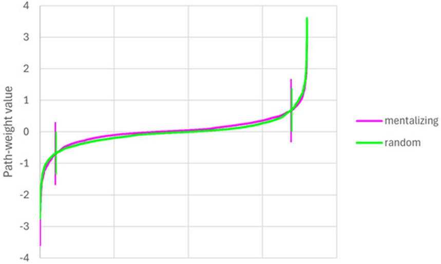
Figure 1. Path-weights plotted per output in increasing order for each stimulus category. Vertical lines signal the location of the elbow points.
Following the systematic ranking and plotting of all input pathways, any path-weights located between the positive and negative inflection thresholds were removed. This structural pruning protocol is described with additional technical detail elsewhere [47].
The remaining "pruned network" was subsequently retrained to recalibrate the weight distributions across the modified architecture. During this retraining stage, a grid search was executed to identify the optimized hyperparameter settings; however, this specific search required training only one network per hyperparameter pair, as the base structural weights were fixed without random initialization. For this phase, the optimal hyperparameter pairing was determined to be a learning rate of 0.7 paired with a momentum value of 0.1. The primary purpose of this retraining phase is to permit the sparse network to optimize its remaining weights within the lightened topography, enabling the model to recover the classification accuracy lost during the pruning step. This secondary optimization stage is expected to achieve greater computational efficiency than the initial training run, given that uninformative features have been permanently excised. This step yields the final "retrained network".
The estimation of the Shapley values is conducted using the retrained network within a Python environment, leveraging the SHAP library (https://github.com/shap/shap) (accessed on 7 October 2024). SHAP serves as an acronym for SHapley Additive exPlanations. Because the baseline network is initially programmed in R using the AMORE package, the architecture must be ported into Python via the PyTorch framework (https://pytorch.org/) (accessed on 7 October 2024). Consequently, a tailored activation function is programmed to replicate the mathematical behavior of AMORE’s tansig function. To transfer the model from R to Python, an identical network topography is initialized in Python via PyTorch, featuring 360 input units, 1 hidden layer containing 10 hidden units driven by the custom tansig activation function, and 5 output units governed by the sigmoid activation function, initialized with arbitrary starting weights. The trained weights extracted from the retrained R network are then mapped into the PyTorch framework using compatible formatting structures, substituting the randomized baseline values. This workflow yields an exact replication of the R-based neural network within Python. The explanation phase is subsequently executed via the SHAP toolkit. An explanatory model is constructed utilizing the DeepExplainer function, which acts as an optimized iteration of the DeepLIFT framework [48]. As detailed in [49], this function approximates the conditional expectations of Shapley values by performing integrations across a comprehensive distribution of samples, such that their summation equals the net difference between the baseline expected output and the true model prediction. The SHAP framework utilizes these approximated Shapley values to organize the input features based on the specific variance they introduce to the model’s prediction; this establishes their respective functional weighting inside the decision pipeline. This analytical sequence generates a distinct score for every input feature, across every individual instance, for each target category. These derived scores can subsequently be averaged by absolute value to establish a unified global ranking of feature importance. Evaluating the direct correspondence between the SHAP value and the base input metric determines whether an individual feature drives a classification pathway positively or negatively; this indicates whether elevated input signals push the model toward selecting that explicit target category or assist the network in ruling out that category.
The empirical findings relating to the SNN-based data modeling and its corresponding interpretations via explainability platforms are detailed first. Subsequently, the outputs generated by the conventional GLM statistical modeling are presented to establish an analytical baseline for direct comparison.
The operational performance metrics across all three network variations are detailed in Table 1. This table outlines the confusion matrices, category-specific precision values (local), and classification accuracies (both local and global scales) for the optimized baseline, pruned, and retrained networks. The cumulative number of accurate classifications reached 75, 68, and 72 (out of a maximum ceiling of 85 test trials), respectively. Thus, the pruned model demonstrates a marginal performance drop, which is successfully mitigated following the retraining protocol. The baseline global classification accuracy was recorded at 88.2%, which decreased to 80.0% upon network pruning. Post-retraining adjustments successfully restored the global accuracy metric to 84.7%.
Table 1. Confusion matrices, precisions, and accuracies of the best, pruned, and retrained networks.
Fully Connected Neural Network |
|
|
|
Input Category | Predicted: mnt | Predicted: rnd | Total Samples |
mnt | 43 | 2 | 45 |
rnd | 8 | 32 | 40 |
Total | 51 | 34 | 85 |
Performance Metric | mnt (%) | rnd (%) | Overall (%) |
Classification Accuracy | 95.6 | 80.0 | 88.2 |
Positive Predictive Value (Precision) | 84.3 | 94.1 | |
Pruned Neural Network |
|
|
|
Input Category | Predicted: mnt | Predicted: rnd | Total Samples |
mnt | 41 | 4 | 45 |
rnd | 13 | 27 | 40 |
Total | 54 | 31 | 85 |
Performance Metric | mnt (%) | rnd (%) | Overall (%) |
Classification Accuracy | 91.1 | 67.5 | 80.0 |
Positive Predictive Value (Precision) | 75.9 | 87.1 | |
Retrained Neural Network |
|
|
|
Input Category | Predicted: mnt | Predicted: rnd | Total Samples |
mnt | 41 | 4 | 45 |
rnd | 9 | 31 | 40 |
Total | 50 | 35 | 85 |
Performance Metric | mnt (%) | rnd (%) | Overall (%) |
Classification Accuracy | 91.1 | 77.5 | 84.7 |
Positive Predictive Value (Precision) | 82.0 | 77.5 |
Evaluating local accuracy parameters—defined as the ratio of valid classifications relative to the total number of experimental trials within a specific task category—reveals that accuracies for the mentalizing (mnt) condition are consistently elevated compared to the random motion (rnd) condition. This trend remains stable across every phase of the network modification lifecycle. It is also important to note that the local accuracy for the mnt classification stays identical between the pruned and retrained configurations; this indicates that the observed recovery in global classification accuracy following retraining is primarily driven by the model restructuring its parameters to better classify rnd events.
Category-specific precision represents the proportion of true positive classifications relative to the total number of positive assignments generated by the model for that group. These precision scores trace a parallel developmental curve to the accuracy metrics, experiencing a decline during pruning and subsequent restoration through retraining. However, while the baseline fully connected architecture demonstrated superior precision for the rnd class compared to the mnt class, this relationship is inverted following the execution of the retraining phase.
To preserve the clarity and focus of the model interpretation, the analytical scope was restricted to the 20 highest-ranked SHAP parameters within each target group. Because this modeling represents a binary classification task, sorting the input data by the mean absolute value of the calculated Shapley profiles yields an identical ordering for both behavioral categories. Figures 2 and 3 present beeswarm distributions highlighting the top twenty input features mapped across both task groups. These neuroanatomical regions provide symmetrical data inputs across categories: if a specific feature registers a positive contribution toward the mnt target, it produces an equivalent negative pull toward the rnd target, and vice versa. Specifically, cortical areas 125, 219, 13, 175, 151, 96, and 159 (arranged in descending sequence based on the modulus of their SHAP values) deliver a positive contribution toward the rnd designation, whereas cortical structures 145, 310, 80, 343, 17, 142, 140, 153, 66, 150, 316, 358, and 120 demonstrate a positive driving force for the mnt designation. Table 2 provides exhaustive regional parameters for each cortical area, specifying its formal nomenclature, spatial layout within the brain, and the corresponding absolute modulus of its SHAP value.
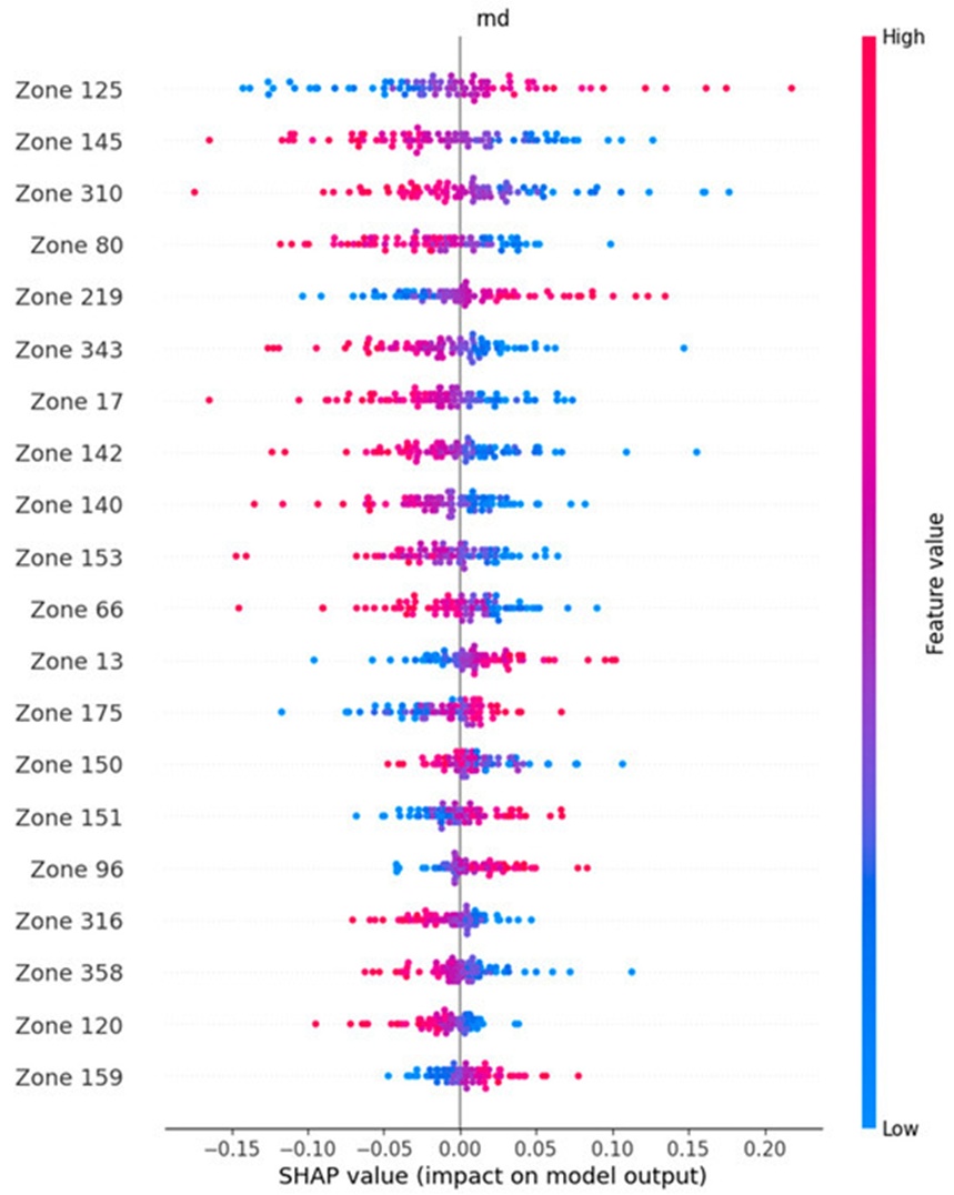
Figure 2. Beeswarm plot depicting the brain regions that hold important information for correct classification in the random class (rnd), ordered by decreasing SHAP value modulus. The brain regions at the top, containing red plots on the right, hold information that, if absent during the calculation of the SHAP value, leads to a drop in the classification performance; thus, such regions are the most important in the classification process.
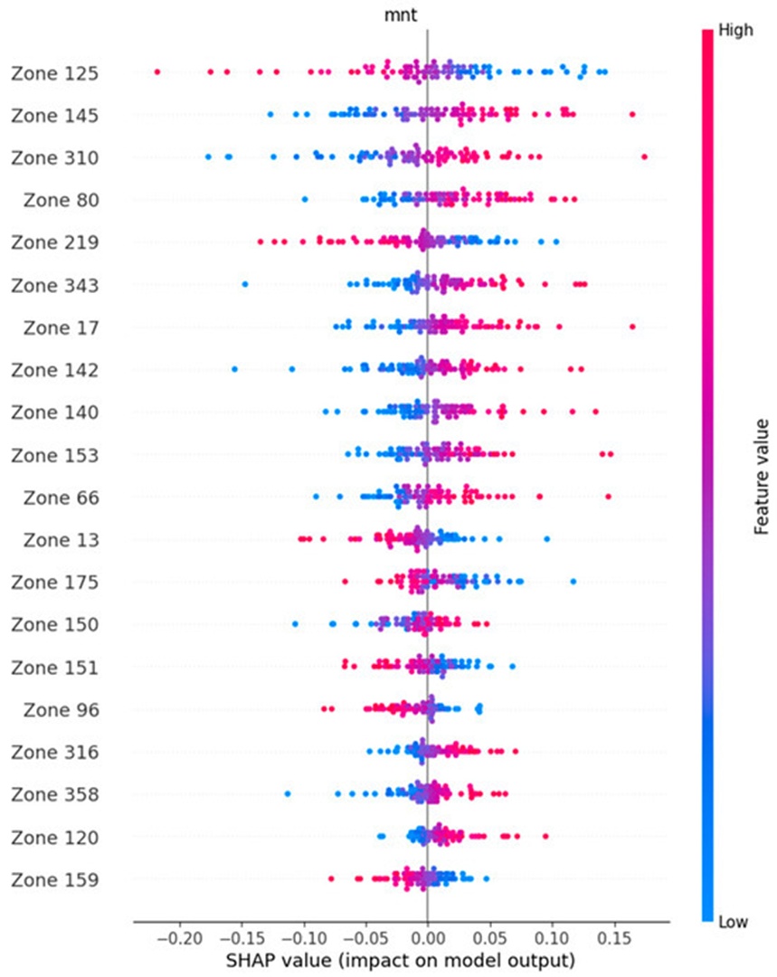
Figure 3. Beeswarm plot depicting the brain regions that hold important information for correct classification in the mentalizing class (mnt), ordered by decreasing SHAP value modulus. The brain regions at the top, containing red plots on the right, hold information that, if absent during the calculation of the SHAP value, leads to a drop in the classification performance; thus, such regions are the most important in the classification process.
Table 2. Brain regions that hold important information for the classification process in this study. Their absence during the Shapley values estimation implicates an important drop in the classification performance. The top section identifies the brain regions holding important information for the random stimuli class, and the bottom section identifies the regions important for the mentalizing task.
Region Identifier | |SHAP| Value | Brain Region | Hemisphere | Cerebral Lobe | Cortex Identifier | Cortical Classification |
Random Stimuli (rnd) | ||||||
96 | 1.506 | Anterior Area 6 L | Left | Fr | 8 | Premotor Cortex |
175 | 1.824 | Auditory Complex 4 L | Left | Temp | 11 | Auditory Association Cortex |
125 | 3.977 | Auditory Complex 5 L | Left | Temp | 11 | Auditory Association Cortex |
151 | 1.580 | Area PGs L | Left | Par | 17 | Inferior Parietal Cortex |
13 | 1.928 | Visual Area V3A L | Left | Occ | 3 | Dorsal Visual Stream |
219 | 2.800 | Visual Area V3B R | Right | Occ | 3 | Dorsal Visual Stream |
159 | 1.357 | Lateral Occipital Area 3 L | Left | Occ | 5 | MT+ Complex and Adjacent Visual Areas |
Mentalizing (mnt) | ||||||
66 | 2.182 | Area 47m L | Left | Fr | 20 | Orbital and Polar Frontal Cortex |
80 | 2.932 | Area IFJp L | Left | Fr | 21 | Inferior Frontal Cortex |
310 | 3.366 | Piriform Cortex R | Right | Temp | 12 | Insular and Frontal Opercular Cortex |
120 | 1.379 | Hippocampus L | Left | Temp | 13 | Medial Temporal Cortex |
17 | 2.590 | Intraparietal Sulcus Area 1 L | Left | Par | 3 | Dorsal Visual Stream |
140 | 2.277 | Temporo-Parieto-Occipital Junction Area 2 L | Left | Par | 15 | Temporo-Parieto-Occipital Junction Cortex |
145 | 3.748 | Intraparietal Area 1 L | Left | Par | 17 | Inferior Parietal Cortex |
316 | 1.440 | Area PFt R | Right | Par | 17 | Inferior Parietal Cortex |
150 | 1.591 | Area PGi L | Left | Par | 17 | Inferior Parietal Cortex |
343 | 2.594 | Area PGp R | Right | Par | 17 | Inferior Parietal Cortex |
153 | 2.188 | Ventromedial Visual Area 1 L | Left | Occ | 4 | Ventral Visual Stream |
358 | 1.439 | Area V3CD R | Right | Occ | 5 | MT+ Complex and Adjacent Visual Areas |
142 | 2.440 | Dorsal Transitional Visual Area L | Left | Occ | 18 | Posterior Cingulate Cortex |
The partial dependence trends illustrated in Figures 4 and 5 mirror the functional alignments described above. Every parsed feature shows highly symmetrical slope trends when compared across the mentalizing and random motion processing paths. Features characterized by steeper coordinate slopes correspond directly with enhanced SHAP outputs, highlighting their heightened importance for achieving successful class assignment. Figure 6 provides a bar chart detailing the top twenty input features, plotted exclusively using absolute SHAP metrics to present an overview independent of feature polarity. This bar chart corroborates that the absolute SHAP influence score for each individual feature remains uniform between both processing categories, displaying variance only in its positive or negative orientation.
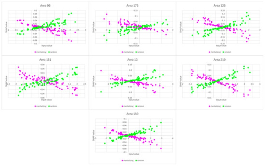
Figure 4. Partial dependence plots for areas 96, 175, 125, 151, 13, 219, and 159. These regions are the ones identified as having the most positive impact toward a classification as random. A positive slope indicates a positive contribution toward the classification as a class, while a negative slope indicates a negative contribution toward the classification as a class. A steeper slope indicates a more important contribution toward the decision, while a flatter slope indicates a less important contribution toward the decision.
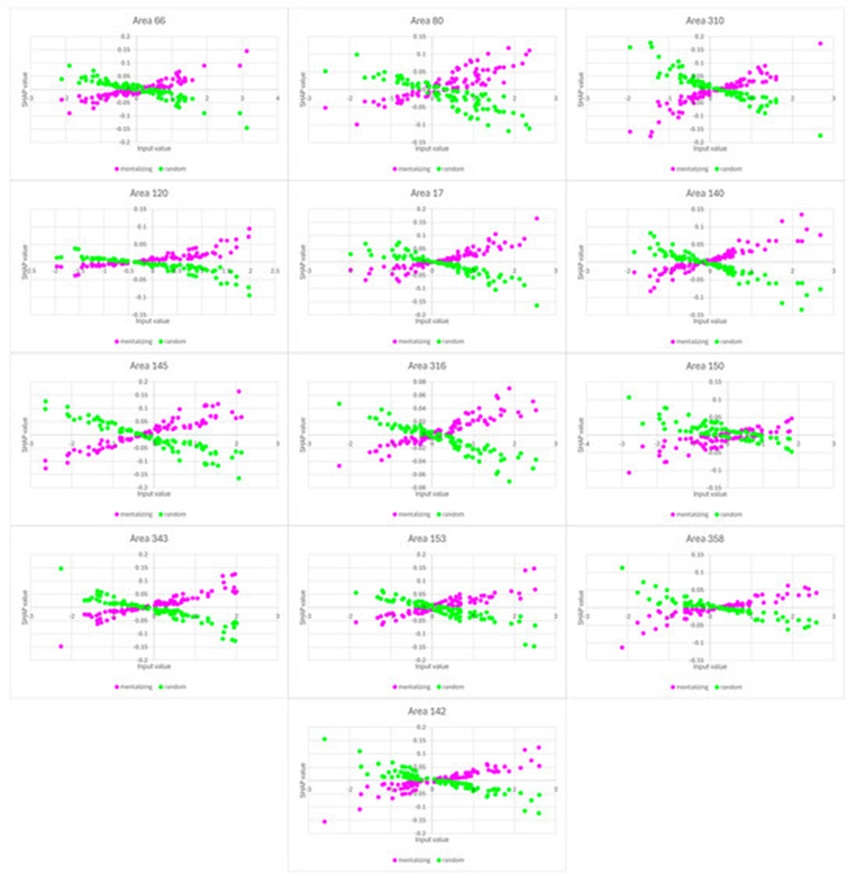
Figure 5. Partial dependence plots for areas 66, 80, 310, 120, 17, 140, 145, 316, 150, 343, 153, 358, and 142. These regions are the ones identified as having the most positive impact toward a classification as mentalizing. A positive slope indicates a positive contribution toward the classification as a class, while a negative slope indicates a negative contribution toward the classification as a class. A steeper slope indicates a more important contribution toward the decision, while a flatter slope indicates a less important contribution toward the decision.
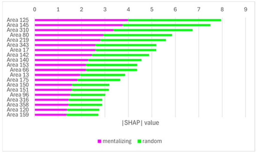
Figure 6. Bar plot of the absolute SHAP values of the twenty top brain areas considered for the focused evaluation. The areas closer to the top are preponderant in the model’s decision. The width of each colored segment is proportional to the SHAP value. However, this graph does not represent polarity.
Figure 7 maps the spatial coordinates of the twenty most critical cortical regions determined by the SHAP analysis, corresponding with the anatomical items indexed in Table 2. Evaluating the mentalizing (mnt) conditions highlights a clear recruitment of cortical regions situated within the bilateral parietal lobes, showing a distinct left-hemispheric dominance, alongside sub-components linked to both the dorsal and ventral streams of the visual processing hierarchy (Figures 7b–7e). Concurrently, several structural zones located within anterior prefrontal regions, specifically bordering the frontal operculum and orbitofrontal networks, are also active (Figure 7a).
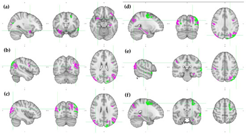
Figure 7. HCP MMP1.0 brain regions with the twenty higher SHAP values modulus (identified in Table 2) depicted over the ICBM152 brain template. The brain regions that are more important for mentalizing (mnt) classification are colored in fuchsia, while those that are more important for random (rnd) classification are green. Each pane contains a sagittal, coronal, and axial view of (a) x = 32, y = 8, z = −16; (b) x = −46, y = −62, z = 24; (c) x = 42, y = −74, z = 26; (d) x = −26, y = −76, z = 34; (e) x = −56, y = −28, z = 40; and (f) x = −24, y = −8, z = 54. MNI152 standard space. Radiological convention. A: anterior; I: inferior; L: left; P: posterior; R: right; S: superior.
The anatomical networks recruited during the random motion (rnd) baseline task display a more diffuse configuration across the cerebrum. While these features occupy positions within the occipital and parietal lobes (Figures 7b–7d), they additionally integrate primary motor and premotor zones (Figures 7d and 7f) alongside extensions into the temporal lobe structure (Figure 7e).
Figure 8 illustrates the patterns of statistical activation and deactivation obtained via the GLM-based processing. In this context, activations represent the directional contrast of mentalizing > random, whereas deactivations correspond to the inverse contrast (random > mentalizing). For both stimulus conditions, these metabolic alterations are distributed across numerous cortical structures. Pronounced activations are observed within multiple regions of the occipital and parietal lobes, localized primarily within ventral areas (Figure 8a–8c), and extending into the fusiform gyri of the temporal lobe (Figure 8a). Additionally, significant clusters of activation are present bilaterally within both the frontal operculum and the medial prefrontal cortex.
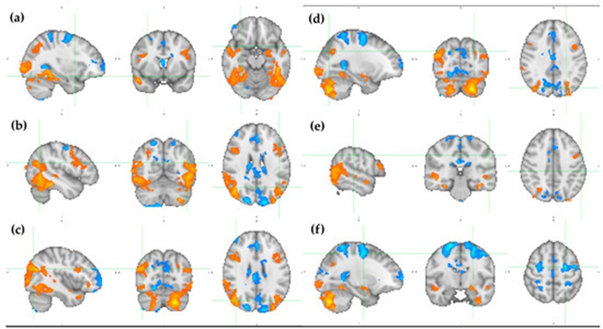
Figure 8. Statistical parameter maps resulting from the GLM-based analysis over the ICBM152 brain template. The activations for mentalizing (mnt) classification are colored from red to yellow (2.3 < z < 6.5), while the deactivations for random (rnd) classification are colored from dark to light blue (-2.3 > z > -6.5). Each pane contains a sagittal, coronal, and axial view of (a) x = 32, y = 8, z = -16; (b) x = -46, y = -62, z = 24; (c) x = 42, y = -74, z = 26; (d) x = -26, y = -76, z = 34; (e) x = -56, y = -28, z = 40; and (f) x = -24, y = -8, z = 54. MNI152 standard space. Radiological convention. A: anterior; I: inferior; L: left; P: posterior; R: right; S: superior.
Significant deactivations are tracking along the cortical zones bounding the longitudinal fissure, specifically spanning caudal, medial, and anterior coordinates (Figures 8b–8d, 8f). The identified medial locations intersect with premotor and motor systems, corresponding prominently to the somatotopic representations of the feet (Figures 8a,8c and 8d) and the hands (Figure 8f).
Figure 9 provides a direct comparative overlay of the localized neuroanatomical maps derived from the post-hoc SHAP analysis alongside the statistical parametric maps generated by the standard GLM workflow. The threshold limits applied to both modalities are selected arbitrarily. For the SHAP model, the analytical scope is restricted to the twenty anatomical regions exhibiting the highest absolute SHAP value modulus; for the GLM analysis, the statistical thresholding is established at z = 2.3 for activations and z = -2.3 for deactivations. It is critical to recognize that these thresholding profiles directly influence the spatial dimensions of the identified clusters.
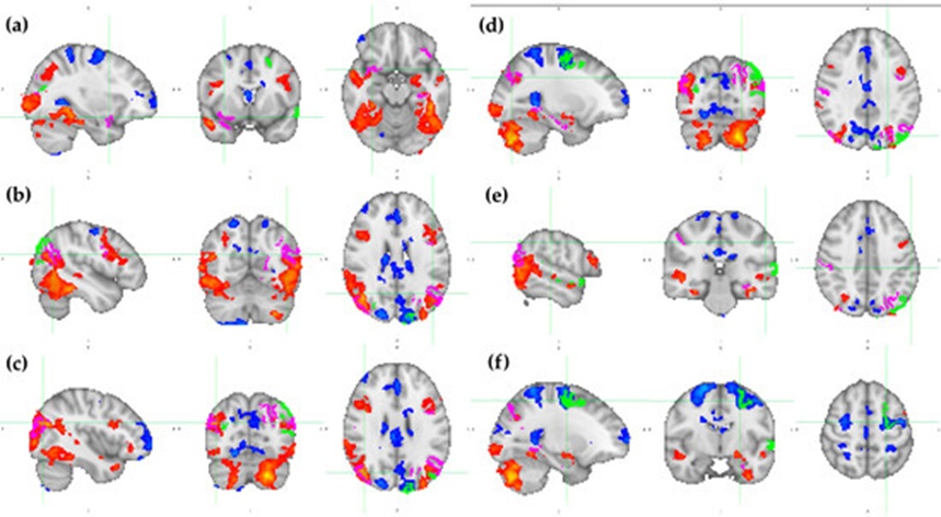
Figure 9. Overlap of the HCP MMP1.0 brain regions with the twenty higher SHAP values modulus (identified in Table 2) over the statistical parametric maps that resulted from the GLM-based analysis. The HCP MMP1.0 brain regions that are more important for mentalizing (mnt) classification are colored in fuchsia, while those that are more important for random (rnd) classification are green. The activations for mentalizing (mnt) classification are colored from red to yellow (2.3 < z < 6.5), while the deactivations for random (rnd) classification are colored from dark to light blue (-2.3 > z > -6.5). Each pane contains a sagittal, coronal, and axial view of (a) x = 32, y = 8, z = -16; (b) x = -46, y = -62, z = 24; (c) x = 42, y = -74, z = 26; (d) x = -26, y = -76, z = 34; (e) x = -56, y = -28, z = 40; and (f) x = -24, y = -8, z = 54. MNI152 standard space. Radiological convention. A: anterior; I: inferior; L: left; P: posterior; R: right; S: superior.
With respect to the mentalizing (mnt) paradigm, widespread spatial convergence is observed across the occipital and parietal lobes (Figures 9b–9e). However, while the GLM statistical clusters are localized more ventrally, the structural domains characterized by elevated SHAP metrics exhibit a dorsal and anterior shift, thereby tracking more extensively into parietal structures (Figures 9a–9d). Within the prefrontal cortex, spatial overlap is absent under these specific thresholding criteria. In the right hemisphere, the feature selected by the SHAP framework is positioned within the frontal operculum, whereas the corresponding GLM statistical cluster resides within the temporal lobe. In the left hemisphere, the SHAP-derived cortical zone appears in isolation, lacking a corresponding statistical cluster underneath (Figure 9a).
For the random motion (rnd) baseline task, a clear spatial convergence is identifiable within the primary hand motor area of the left hemisphere, though this effect does not emerge in the right hemisphere, as illustrated in Figure 9f. Notably, the remaining statistical deactivations do not exhibit spatial overlaps with the SHAP-derived regions. Furthermore, the targeted SHAP features located within the occipital and parietal lobes lack corresponding statistical deactivations in the GLM model.
The computational framework evaluated in this investigation was previously validated utilizing task-based motor fMRI paradigms extracted from the HCP database [5]. However, extending the validation of this technique to a higher-order cognitive framework introduces enhanced technical challenges and establishes a pathway for broader, more sophisticated neuroscientific applications. Explainability tools, in particular, can be deployed to uncover important insights regarding underlying neurocomputational processes. By isolating the specific cortical regions leveraged by the network to differentiate between distinct stimulus conditions, it becomes possible to map the functional topologies driving the cognitive paradigm. This framework of functional connectivity has been extensively evaluated for the classification and clinical forecasting of neuropsychiatric disorders, such as schizophrenia, bipolar disorder, autism spectrum conditions, attention deficit hyperactivity disorder, Alzheimer’s dementia, and mild cognitive impairment [12].
Complex cognitive paradigms highlight some of the primary limitations of conventional GLM analysis. The GLM methodology exhibits two prominent operational constraints. First, it relies on the mathematical assumption of linear independence among input signal sources to guarantee that the underlying design matrices remain invertible—a condition that cannot be confidently assumed during higher-order cognitive processing. Second, because its mathematical foundation relies on linear regression, it assumes that the neurophysiological impacts of paradigm manipulations interact in a purely summative manner. However, human brain activity often operates via non-linear dynamics; consequently, experimental task manipulations may induce network interactions that are far more complex than simple additive effects. In contrast, the SNN-based workflow introduces no such rigid assumptions regarding the independence of fMRI source signals. Indeed, the integration of non-linear activation functions such as "tansig" and "sigmoid" enables the model to characterize the underlying neural dynamics with greater fidelity.
The baseline predictive performance of the network exceeded the classification accuracies previously achieved in motor mapping studies, reaching 88.2%, which is substantially above statistical chance. While a decrease in predictive accuracy is expected during the connection pruning phase, the subsequent recovery of classification performance demonstrates that the connection weights of the surviving architecture are effectively recalibrated to offset the reduced volume of input features used for class assignment.
The functional explanations generated by the SHAP framework show strong convergence with established neuroscientific models of the cortical networks driving Theory of Mind. Neuroimaging literature focused on ToM consistently implicates the medial prefrontal cortex (mPFC) [50-52], the temporoparietal junction (TPJ) [51, 53-55], the superior temporal sulcus (STS) [50, 52, 56], and the inferior frontal gyrus (IFG) [57] as core components of the neural network enabling individuals to infer and evaluate the internal mental states of social counterparts—a system required for proficient social cognition and navigation. The close alignment between these historically verified regions and the top features identified by the SHAP framework confirms this coherence.
Nevertheless, concerning the SHAP-derived interpretations, it is critical to note that this explanatory framework may not capture every anatomical area involved in task execution. Although the isolated regions are directly utilized by the model to partition the behavioral classes accurately, the atlas-based parcellation scheme is strictly structural and operates independently of the functional signal variations within those zones; consequently, certain areas may exhibit highly correlated BOLD profiles. Due to the mathematical characteristics of artificial neural networks, when configured with collinear or redundant features, the optimization algorithm may arbitrarily prioritize one input channel over another (often dictated by the initial randomized weight parameters). As a result, certain highly relevant task-related features may be discarded during the pruning phase because the network is capable of extracting equivalent predictive information from alternative channels. Within these sets of co-varying, task-relevant inputs, only a subset may persist into the final network architecture and register sufficiently high Shapley coefficients to appear in the top-ranked visualizations.
Nonetheless, this analytical workflow successfully yielded a parsimonious, interpretable, and explainable computational model capable of accurately classifying data from a complex, cognitive fMRI paradigm. The generated explanations align with foundational Theory of Mind research and support robust neuroscientific interpretation. This fMRI processing pipeline effectively bypassed the limitations of traditional models when applied to a cognitive task, demonstrating strong performance and yielding meaningful explanations despite the highly complex and non-linear properties of the underlying neural processes. Consequently, post-hoc explainability frameworks implemented on SNN architectures offer a highly effective tool for knowledge extraction within functional neuroimaging analysis. The insights derived from these workflows hold significant promise for advancing clinical mental health research and neural state decoding applications.
The empirical outcomes achieved in this study point toward a promising path for the engineering of interpretable digital twins of the human brain, offering substantial utility for the clinical diagnosis of psychiatric and neurological conditions. Mapping the explicit functional topologies underlying these disorders can facilitate the engineering of highly targeted, patient-specific therapeutic interventions, which may demonstrate enhanced clinical efficacy relative to current standard protocols.
Subsequent research must investigate how multi-collinearity and linear dependence among features influence the retention or elimination of specific cortical inputs during the network pruning process. Developing a thorough mathematical understanding of why certain linearly correlated features are designated as highly important by the network while others are omitted as redundant will allow for a more complete decoding of the network's internal decision logic and, by extension, a more complete mapping of true brain function.
An additional area of investigation involves embedding domain-specific biological constraints directly into the neural network architecture. At present, the computational model assumes that signal propagation between separate cortical targets occurs homogeneously. However, the human brain is organized as a complex small-world network wherein long-range white matter tracts allow specific regions to exchange information rapidly across great physical distances, while intervening cortical structures require longer temporal windows for signal transmission. Because these topological heterogeneities directly shape functional connectivity profiles, subsequent iterations of this framework must transition from standard tabular data structures to alternative graph-based representations that more accurately capture the non-Euclidean geometry of neural information transfer.
None
None
The authors declare that financial support was received for the research, authorship, and publication of this article. This work was financially supported by Base Funding UIDB/00027/2020 of the Artificial Intelligence and Computer Science Laboratory, LIACC, funded by national funds through the FCT/MCTES (PIDDAC). NECE-UBI, Research Centre for Business Sciences, Research Centre, and this work are also funded by FCT, Fundação para a Ciência e a Tecnologia, IP, project UIDB/04630/2020.
None
Open Access The author(s) retain copyright. This article is licensed under the Creative Commons Attribution-NonCommercial-ShareAlike 4.0 International License. It may be shared and adapted for non-commercial purposes with appropriate attribution, an indication of changes, and distribution of adaptations under the same license. Third-party material may be subject to separate terms identified in its credit line. View the license at https://creativecommons.org/licenses/by-nc-sa/4.0/.
 Transparent Intelligence Publishing