The reliability and security of convolutional neural networks (CNNs) have attracted growing attention, particularly in domains where safety is paramount, such as clinical medicine. Even though CNNs demonstrate high competency in categorizing images, their outcomes frequently exhibit vulnerability to minor image adjustments that remain imperceptible to human observers. Consequently, an altered, degraded image can appear identical to the authentic image to a person, yet mislead the CNN into making an incorrect classification. Throughout this study, these altered images are termed adversarial images. A widespread approach for producing adversarial images involves propagating the loss gradient backward to alter the source image. Typically, perturbations have been established using solely the gradient direction and a fixed step size (referred to as the fast gradient sign method, or FGSM), or by executing the FGSM iteratively to craft more potent perturbations capable of altering the model's categorization (i-FGSM). Conversely, if the step size is excessively large, the smallest possible image perturbation might be overlooked during the gradient exploration. To discover precise and minimal input image variations necessary to prompt a classification shift, this paper proposes initiating the FGSM with a small step size and dynamically tuning it across iterations. For evaluation, several decay algorithms from existing literature were assessed against a novel method driven by an index monitoring the state of the loss. Ultimately, three separate tracking functions were implemented for comparative analysis. The empirical findings demonstrate that our loss-adaptive decay algorithms successfully identified adversarial examples with a success rate exceeding 90% while introducing fewer distortions to mislead the CNNs.
Convolutional neural networks (CNNs) are widely utilized for executing image recognition assignments because they possess the capability to automatically extract visual features from images or video content. In historical investigations, these visual characteristics were predominantly crafted manually, which introduces the risk of omitting vital information during the feature extraction phase [1]. CNNs bypassed these constraints and substantially enhanced the efficiency of image classification. Nonetheless, the efficacy of CNNs is heavily dependent on image quality, target visibility, and additional variables present during the training phase [1]. For example, in clinical settings—such as identifying surgical instruments within laparoscopic surgery video feeds—specific visual difficulties strongly impact the classification performance of CNNs [1, 2]. These visual difficulties occur frequently in practical medical scenarios; for instance, surgical instruments can be hidden by anatomical tissue, smoke may develop during operative procedures, lenses can become obscured by blood, and motion blur can arise from rapid actions or an unstable camera setup [1]. These impediments jeopardize the performance of CNNs, obstructing the accurate identification of surgical instruments under challenging conditions. Furthermore, even a highly trained CNN can be readily disrupted by minor adjustments introduced to authentic images, and this susceptibility to adversarial instances is a shared characteristic across all CNN frameworks [2-6]. Consequently, dedicated research is required to strengthen the resilience of these models against adversarial perturbations.
Adversarial images can be easily produced by mirroring the image [7] or by introducing imperceptible alterations to the original input [3-6, 8]. An effective, targeted strategy for crafting adversarial image perturbations involves the backpropagation of the loss gradient to serve as a directed modification to the input images [3-6, 8, 9]. The fast gradient sign method (FGSM) was initially introduced in [9] and subsequently modified through various extensions, such as repeatedly applying the FGSM to the input [10], incorporating momentum into the gradient calculation (MI-FGSM) [11], or mapping the perturbation back onto a max-norm boundary after each iteration (PGD) [12]. Additional methodologies have been detailed in the literature, including utilizing the forward derivative to formulate adversarial saliency maps [13] or employing generative adversarial networks (GANs) [14].
To evaluate the resilience of convolutional neural networks against these adversarial images, a max-norm constraint is typically enforced on the perturbation amplitude. A high error frequency on these adversarial images signifies diminished robustness in the classification performance of the convolutional neural network. Generally, an escalation in perturbation amplitude leads to an increase in the error rate. However, the inverse perspective—a metric centered on the minimal perturbation required to compel a model to misclassify an input—represents another compelling research path. Relevant studies exist in the literature, such as developing provably minimally distorted adversarial instances via formal verification methods [15], utilizing fast adaptive boundary attacks to craft minimally distorted adversarial examples [16], employing a highly constrained framework that modifies only a single pixel as introduced in [17], designing an optimization framework to produce an adversary with an adjustable amplitude [18], and utilizing an adaptive learning rate to modulate the modification process [19].
The main contributions of this paper are detailed below:
We introduce the step size adaptive i-FGSM to generate adversarial examples utilizing smaller perturbations. At the start, the standard fast gradient sign method (FGSM) was utilized to identify a minimal perturbation tailored to each separate input that suffices to alter the model's output. If the magnitude of the perturbation is insufficient to shift the prediction, the procedure transitions into an iterative format (i-FGSM) until misclassification is achieved. This strategy is somewhat unrefined and frequently fails to yield an optimal minimal solution. Thus, we adjusted this minimum exploration process and framed it as an adaptive gradient descent problem [19]. To resolve this issue, this study builds further upon the methodology established in our prior work [19].
We present a loss-adaptive framework designed to modulate the step size. Three distinct decay algorithms sourced from the literature were applied to regulate the step size (or the learning rate within a machine learning context). Furthermore, we present an original decay algorithm that monitors the loss of the current iteration and utilizes this data as feedback to modulate the step size for the subsequent iteration. In total, three distinct loss-tracking functions are utilized: the loss rescale function, the loss trigonometric function, and the loss-related original classification probability.
We deliver experimental outcomes demonstrating the impact of varying step sizes on the adversarial generation procedure. The empirical study is split into two segments depending on whether a specific target class is assigned. Specifically, an adversary can be created either by shifting the input away from its true classification or by driving the input closer to a designated target classification. The experimental findings reveal that our loss-adaptive step size algorithms can successfully produce adversaries with reduced perturbations while sustaining a high rate of adversarial success.
In this investigation, our primary dataset is the Cholec80 dataset [1], which comprises 80 videos of cholecystectomy procedures utilizing 7 distinct surgical instruments (illustrated in Figure 1), establishing 7 separate categories (Table 1) for detection within the video frames [19-22]. To satisfy the SoftMax criteria [23], image frames containing only 1 class are utilized in this work and were isolated from the dataset (totaling 80,190 images). From this compiled dataset, the initial 40 videos (containing 31,477 images) served as the training corpus, while the remaining 40 videos (containing 48,713 images) functioned as the evaluation test set. The convolutional neural network architecture utilized as a representative model in this investigation is Resnet-50 [24]. Resnet-50 incorporates a basic baseline network that initiates with down-sampling convolutions followed by four convolutional blocks, terminating with an average pooling layer, a fully connected layer, and a SoftMax layer. Shortcut connections were integrated into the basic network to implement the residual learning structural adaptation [24]. The architecture underwent training for 30 epochs. To evaluate adversarial perturbations, 200 accurately classified images from each category were selected at random from the test set, resulting in a total of 1400 images for experimentation.
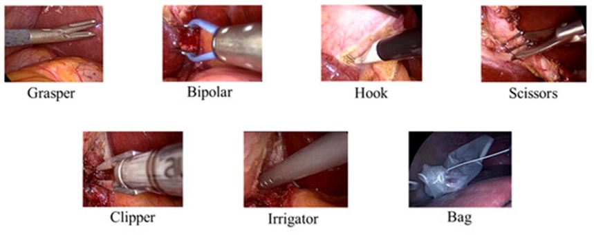
Figure 1. The 7 surgical tools used in the Cholec80 dataset [1].
Table 1. The class index, corresponding surgical tool, and the number of frames in the derived 1-class dataset.
Class | Surgical Tool | Number of Frames |
1 | Grasper | 23,507 |
2 | Bipolar | 3222 |
3 | Hook | 44,887 |
4 | Scissors | 1483 |
5 | Clipper | 2647 |
6 | Irrigator | 2899 |
7 | Bag | 1545 |
As outlined in the introduction, an enhanced version of the fast gradient sign method was utilized to identify adversarial examples that exhibit the smallest possible distortions. In scenarios where a single-step modification fails to displace the input into an alternative category, the algorithm switches automatically to a standard iterative configuration (i-FGSM) until a shift in the predicted label occurs (Figure 2). For example, the transformation sequence can begin with a small perturbation magnitude and continuously update the input until misclassification is achieved; the difference vector between the baseline input and the resulting adversary defines the absolute minimum successful perturbation for that specific instance. This boundary also delineates a minimal security perimeter enclosing the original data point. Nevertheless, this minimum successful perturbation is not determined solely by the inherent properties of the sample—such as its spatial proximity to a decision boundary—but is also governed by the configuration of the model, specifically how closely it approximates ideal decision boundaries. Inducing misclassification in a highly optimized model is considerably more difficult than doing so in an undertrained counterpart; additionally, distinct network architectures typically demonstrate varying degrees of robustness against these inputs. At the same time, executing a nonlinear optimization within a high-dimensional input space (such as high-resolution images) presents a substantial challenge, as the gradient path is highly susceptible to optimization errors, choice of step size, and entrapment in local minima.
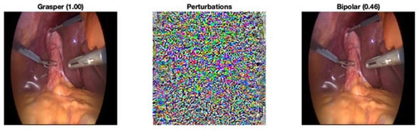
Figure 2. Modify an image from Grasper (class 1) to Bipolar (class 2) with the fast gradient sign method (FGSM). The adversary (right) with minimal perturbation was generated exactly when the classification changed.
From a practical standpoint, mapping the entire decision boundary surrounding a class center to find the absolute shortest distance to an adjacent category is infeasible. Consequently, an approximation method is adopted that evaluates specific vectors within the high-dimensional image space. The targeted adversarial attack employs a gradient search designed to minimize the cross-entropy loss between the network's prediction and a designated target class, effectively driving the image toward the manifold of that selected category [10, 19]. Conversely, a non-targeted adversarial attack maximizes the cross-entropy loss between the model's prediction and the true class, executing a steepest ascent away from the baseline category center [9, 10, 19]. For both methodologies, the resulting modification is intended to represent the closest successful perturbation along that relative trajectory. The cross-entropy loss function is structured as follows:
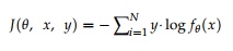 (1)
where 𝜃 signifies the operational model parameters, N denotes the total number of distinct categories, x is the input image provided to the system, 𝑓𝜃(𝑥) is the class probability distribution predicted by the model for x, and y represents the baseline ground-truth label during a non-targeted attack, or the intended destination category label during a targeted attack.
When a specific target category is designated for the adversarial attack [10, 19], the input is iteratively updated by executing gradient descent on (𝜃, 𝑥, 𝑦), where y represents the label of the target class (class(x) ≠ y). The baseline iterative fast gradient sign method (i-FGSM) is expressed as follows:
 (2)
where represents the baseline uncorrupted image, is the synthesized adversarial sample at the nth step, and is the synthesized adversarial sample at the (n − 1)th step. The term 𝑦𝑡𝑎𝑟𝑔𝑒𝑡 denotes the chosen destination label, which cannot match the original class of image x. In this study, α starts as a fixed value and is subsequently transformed into distinct operational functions α(n) that adjust according to the iteration index. In this manner, the step size governing the iterative image updates is regulated via different decay algorithms, allowing for an investigation into how they influence the total perturbation volume required to alter the classification decision. The ultimate perturbation vector, denoted by 𝛿, is obtained by accumulating the incremental adjustments introduced throughout the iterative cycle. The search for the optimal minimum perturbation 𝛿* can be modeled as the nonlinear optimization problem shown in Eq. 3 below, minimizing the geometric distance until the predicted label transitions to the target class.
 (3)
When conducting a non-targeted adversarial attack, the input is updated by ascending the gradient of the original classification loss, thereby forcing the model's prediction into an alternate category [9, 10, 19]. This iterative sequence is defined as follows:
 (4)
In contrast to the targeted attack strategy, this non-targeted optimization seeks to identify any incorrect classification category by driving the cross-entropy loss upward and away from the authentic class 𝑦𝑜𝑟𝑖𝑔𝑖𝑛. This is performed by adding the sign vector of the loss gradient directly to the pixel coordinates. The parameter α(n) is configured to vary dynamically across iterations. Under these criteria, the optimization problem for establishing the smallest perturbation 𝛿* is formulated to minimize the required change while pushing the model past its classification boundary.
 (5)
When using a constant step size \alpha, the magnitude of the image update remains uniform during every iteration; however, as the loss values approach a minimum (Figure 3), this unyielding increment becomes too coarse to isolate an optimal configuration. Consequently, rather than applying a fixed step size at every step, the current state of the loss can provide valuable feedback as a tracking metric to regulate the step size for the subsequent iteration.
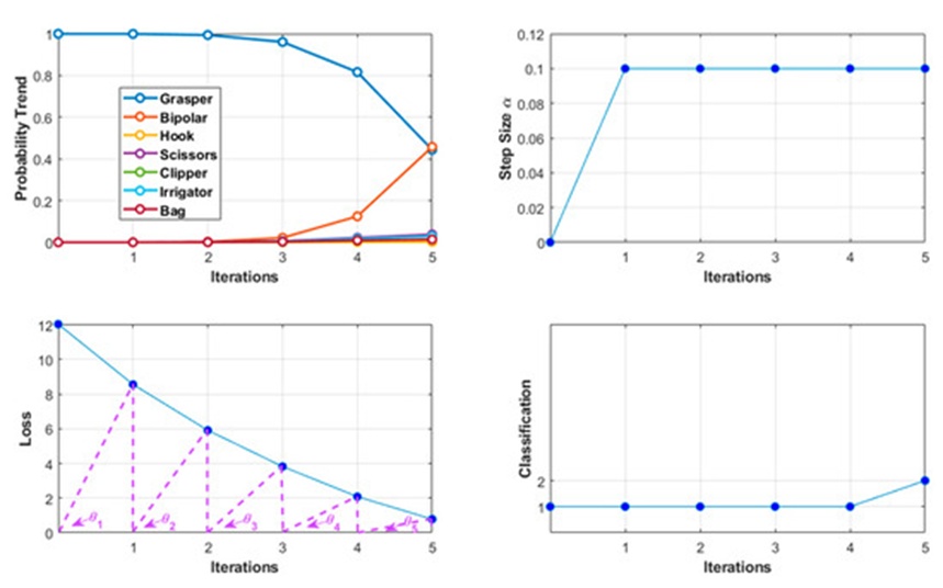
Figure 3. Targeted modification of an image from Grasper (original class yorigin) to Bipolar (target class ytarget) with a constant step size of 0.1. The target classification loss and original class probability are decreasing while the target class probability is increasing. The angles θn in the loss axis are used in the trigonometric functions to describe the loss status.
Although quantifying the exact status of the loss is a complex task, the relationship between the current and prior loss values establishes a trajectory that can roughly project the subsequent loss state. If the perturbed image nears the classification boundary during the optimization process, the step size must decrease to prevent overshooting the boundary. The step size α can be modulated by the loss state by converting this metric into a dynamic decay factor Fn. Three alternative functions are introduced and evaluated here based on their effectiveness and optimization efficiency.
1. Rescale function
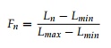 (6)
When a destination class is specified in a targeted adversarial attack, the loss at step (n + 1) can be projected as converging to 0. Consequently, a loss sequence [L1, L2, … Ln, 0] can be rescaled into a normalized vector bounded between 0 and 1, yielding [F1, F2, … Fn, 0]. The variable Fn serves as a scaling factor to scale down the step size, with its magnitude dropping in tandem with the reduction in targeted classification loss.
When attempting to maximize the original classification loss during a non-targeted adversarial attack, the loss at step (n + 1) is instead projected as Ln + 1. The corresponding loss sequence [L1, L2, … Ln, Ln + 1] is then normalized into the vector [F1, F2, … Fn, 1], making the functional decay factor (1 − Fn). In both scenarios, the artificial trailing terms 0 or Ln + 1 are appended solely to anchor the data range, ensuring the immediate loss value behaves as an informative decay controller.
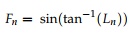
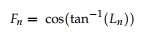
2. Trigonometric functions
Trigonometric formulations can normalize the loss sequence without requiring an external boundary projection, as an operational angle \theta_n is computed at each step to reflect the current loss magnitude (see Figure 3 for the spatial layout of the loss axis).
Thus, as the targeted classification loss drops during a targeted adversarial attack, the step size is adjusted via:
 (7)
When driving up the original classification loss during a non-targeted adversarial attack, the adjustment functions as follows:
 (8)
3. Direct application of original class probability scores
This approach represents an efficient and computationally simple technique for monitoring the immediate state of the loss function.
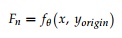 (9)
where 𝑓𝜃(𝑥) is the raw output vector of the model for input x, and 𝑓𝜃(𝑥,𝑦𝑜𝑟𝑖𝑔𝑖𝑛) denotes the specific probability assigned to the authentic baseline category 𝑦𝑜𝑟𝑖𝑔𝑖𝑛.
In addition, the update step size within the i-FGSM framework can be governed by several different scheduling functions [19]. Various standard learning rate attenuation methods are widely documented in optimization literature [25-28], including time-based iteration decay [29], exponential decay [30], and step-wise decay [31]. The complete suite of decay algorithms evaluated in this study is organized in Table 2.
Table 2. The decay functions used in this paper. Where 𝛼,0,𝑛 represent the step size, initial step size, and iteration, respectively.
No. | Learning-Rate Decay Method | Mathematical Expression |
1 | Fixed (Constant) Decay | 𝛼=𝛼0 |
2 | Iterative Decay | 𝛼=𝛼0/(1+0.5(𝑛−1)) |
3 | Exponential Reduction | 𝛼=𝛼0·𝑒(−0.5(𝑛−1)) |
4 | Stepwise Decay | 𝛼=𝛼0·0.5𝑓𝑙𝑜𝑜𝑟((𝑛−1)/1) |
5 | Loss-Based Rescaling |
|
6 | Trigonometric Loss Decay | 𝛼=𝛼0· sin(tan−1(𝐿𝑛)) 𝑜𝑟 𝛼0· cos(tan−1(𝐿𝑛)) |
7 | Probability-Driven Loss Decay | 𝛼=𝛼0· 𝑓𝜃(𝑥,𝑦𝑜𝑟𝑖𝑔𝑖𝑛) |
The effectiveness of a given decay algorithm in altering model predictions is demonstrated by measuring the minimum successful perturbation required. To determine the geometric distance separating the original image from its adversarial counterpart, the L2-norm function was utilized. Typically, the spatial distance between the baseline and adversarial images reflects how challenging it is to alter the model’s classification, where greater distances signify higher model robustness. Consequently, in this study, an algorithm that yields a smaller perturbation to deceive the network is considered more efficient at bypassing the model's defensive mechanisms. It is important to note that certain class instances naturally reside at a greater distance from the decision boundary, which directly impacts the magnitude of the required perturbation. Furthermore, constraints inherent to the optimization approach, such as the characteristics of the decay function, can make identifying an adversarial example more complex. To ensure the computational process terminates, a restriction on the maximum number of iterations was implemented (Algorithm 1). If an input sample cannot be successfully misclassified within 100 iterations, the process is logged as a failure to identify an adversary. Therefore, the adversarial success rate serves as an additional evaluation metric for comparing the performance of the various algorithms.
To evaluate how sensitive the optimization is to the primary step magnitude, three distinct trials were executed with the initial step size 𝛼0 specified as 1, 0.1, or 0.01, respectively.
The upper limit for iterations is set to 100. The iterative process was terminated immediately when the modified image triggered a misclassification during a non-target attack, or when it successfully transitioned into the specified target class during a target attack. Instances exceeding 100 iterations without achieving this are categorized as failures.
The divergence separating the initial baseline image x and the ultimately produced adversarial image 𝑥∗ was quantified utilizing the 𝐿2-norm distance [3-5], which is equivalent to the Euclidean distance, where m denotes the total pixel count.
 (10)
Other standard 𝐿𝑝-norm distance metrics are also applicable, including 𝐿0 distance, 𝐿1 distance, and 𝐿∞ distance [3-5]. Here, the 𝐿0 metric quantifies the total number of altered pixels in 𝑥∗ relative to the baseline image x; the 𝐿1 metric sums the absolute pixel-wise differences across 𝑥∗; and the 𝐿∞ metric identifies the single largest pixel variation within 𝑥∗.
 (11)
The comprehensive architecture of the adversary-generation procedure is outlined systematically in Algorithm 1.
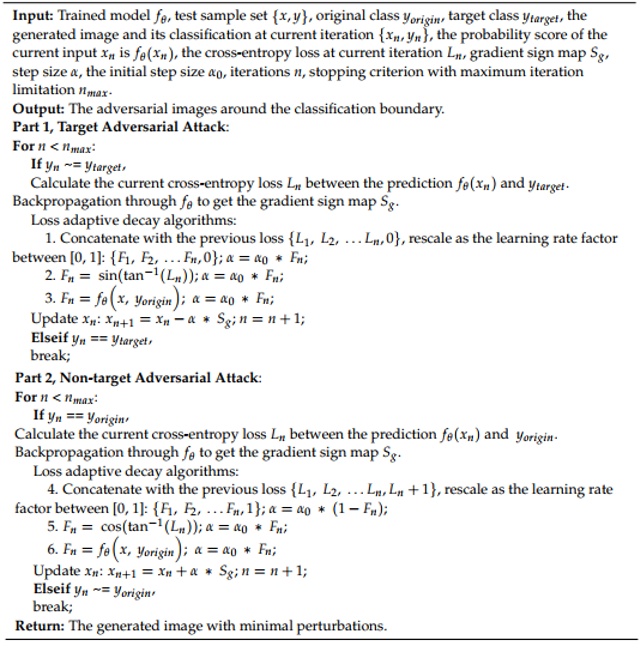
Algorithm 1. Generate adversarial image with adaptive step size
As detailed in the experimental design, diverse decay functions were deployed to identify adversarial examples. Each individual image possesses a distinct ‘smallest perturbation’ bounded by the conditions of the experiment. To evaluate and compare the performance efficiency of these respective decay functions, the average minimum perturbation across all successfully misclassified images was determined. Throughout the target adversarial attack phase, the baseline image is systematically ‘perturbed’ along varying vectors corresponding to the six distinct target classes. The parameter weight space is evaluated across these separate orientations (moving from the true class toward a target decision boundary) by identifying the minimal necessary perturbations.
Figure 4 illustrates the success rate achieved in discovering adversarial examples via the target adversarial attack framework. With the primary step size set to 1 (\alpha_0=1), only the fourth function (step decay) and the seventh function (dependent on the original classification probability) missed the target classification boundary, failing in 10 and 286 instances, respectively. This occurred within a total testing pool of 1400 samples evaluated across six target classes, resulting in 8400 total test cases for the target adversarial attack. When the step size parameter is adjusted downwards to 0.1 and 0.01, the second function (iteration decay), third function (exponential decay), and fourth function (step decay) exhibit a pronounced reduction in success rate. A reduced initial step magnitude combined with a rapid attenuation factor restricts the search speed toward local minima, thereby amplifying the degradation of overall algorithmic efficiency.
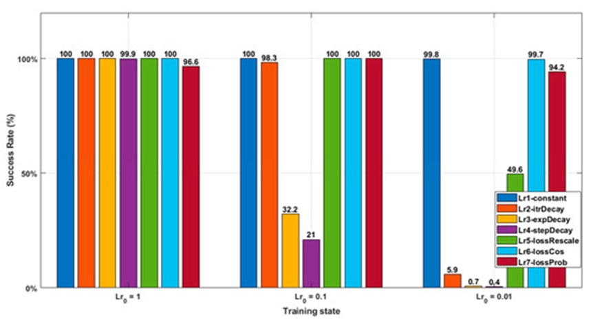
Figure 4. This chart illustrates the proportion of trials that successfully reached the intended misclassification boundary prior to reaching the 100-iteration threshold. The assessed attenuation methods are presented sequentially as constant, iteration-based, exponential, and step-wise decay, followed by three loss-dependent formulations: the scaling, trigonometric, and baseline classification probability functions.
Figure 5 displays the minimum perturbation values required to find target adversaries. The average L2-norm distances were computed exclusively from the pool of successfully generated adversarial examples. At initial learning rates of 1 and 0.1, the first function (constant) and the sixth function (loss trigonometric function) produced larger overall perturbations compared to rival methods, whereas the fifth function (loss rescale function) minimized the required perturbations. When evaluating an initial learning rate of 0.01, the assessment was restricted to just thirty-seven mutually successful instances, given that the fourth function (step decay) demonstrated an exceptionally low success rate for striking the target class within the 100-iteration limit. In this scenario, the calculated perturbations were distributed nearly uniformly, demonstrating that the ultimate solution was dictated predominantly by intrinsic image traits (such as proximity to the decision boundary) rather than the choice of decay algorithm.
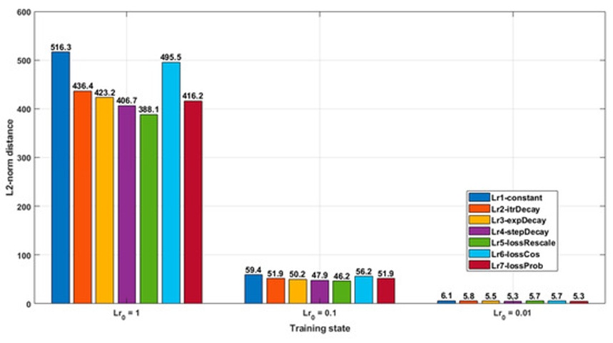
Figure 5. This graph tracks the minimum distortion levels produced by the various adaptive step-reduction methods under a targeted attack framework. Calculations are strictly limited to mutually successful trials across the specified step settings (𝛼0= 1, 0.1, 0.01, yielding 8104, 1768, and 37 overlapping successful instances, respectively). The evaluated strategies are arranged in sequence: constant, iteration decay, exponential decay, step decay, and the final three loss-modulated variants (rescaling, trigonometric, and baseline classification probability).
During the non-target adversarial attack phase, the input sample is dynamically redirected toward the closest available adversarial decision region (Table 3); consequently, this spatial distance is expected to reflect a smaller perturbation than what is observed in target attacks. This non-target adversarial attack configuration evaluated 1400 cases in total, revealing an adversarial discovery success rate that closely mirrors the patterns observed in the target attack trials.
Table 3. This dataset records the geometric proximity to alternative classification zones when utilizing the sixth formulation (loss-based trigonometric variation) within a non-targeted attack environment.
Original Class | Dominant Final Class (𝛼₀ = 1) | Dominant Final Class (𝛼₀ = 0.1) | Dominant Final Class (𝛼₀ = 0.01) |
1 | Class 7 (30.5%) | Class 7 (30.5%) | Class 7 (31.0%) |
2 | Class 1 (60.5%) | Class 1 (61.0%) | Class 1 (60.5%) |
3 | Class 1 (69.0%) | Class 1 (64.5%) | Class 1 (64.5%) |
4 | Class 1 (42.0%) | Class 1 (43.5%) | Class 1 (44.0%) |
5 | Class 1 (51.5%) | Class 1 (46.0%) | Class 1 (46.5%) |
6 | Class 1 (45.0%) | Class 1 (44.5%) | Class 1 (43.5%) |
7 | Class 1 (77.5%) | Class 1 (78.5%) | Class 1 (78.5%) |
When utilizing a baseline step size of 1, a 100% misclassification success rate is achieved across all instances, irrespective of the selected step size adaptation technique. Conversely, at initial step sizes of 0.1 and 0.01, the success rates for the second, third, and fourth decay functions experience a sharp, rapid decline (Figure 6).
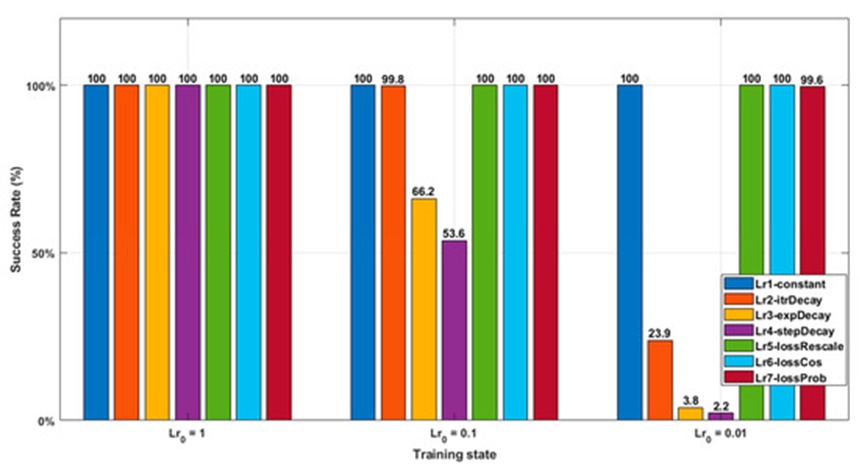
Figure 6. This diagram represents the proportion of runs that successfully completed a non-targeted misclassification within the 100-iteration cap. The specific decay formulations are ordered as constant, iteration-driven, exponential, and step-based, followed by the remaining three loss-driven policies consisting of the scaling function, trigonometric function, and baseline classification likelihood.
The minimum required perturbations exhibit minor variations compared to the target adversarial attack outcomes. As demonstrated in Figure 7, the step decay function consistently yields the smallest perturbation regardless of the starting step magnitude, while the first function (constant) consistently requires the largest; additionally, our three loss-tracking functions generate smaller perturbations than the baseline constant function, yet they require greater perturbations than those produced by the second, third, and fourth decay approaches.
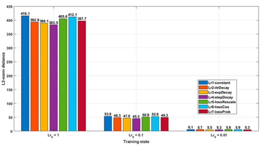
Figure 7. This chart indicates the absolute lowest distortion values generated across different adaptive step-reduction frameworks during non-targeted manipulation. The plotted values incorporate only the mutually successful trials across the step conditions (\alpha_0 = 1, 0.1, 0.01, which map to 1400, 751, and 31 overlapping successes, respectively, out of a grand total of 1400 non-targeted test instances). The seven evaluation approaches are organized in the following order: constant, iteration-based, exponential, step-wise, followed by the loss-dependent scaling, trigonometric, and baseline probability functions.
Based on the experimental outcomes, reducing the primary step magnitude to 0.01 noticeably increased the difficulty of identifying an adversarial classification for the target images. This performance degradation was particularly prominent for the second (iteration-based), third (exponential), and fourth (step-wise) decay strategies. An instance of a highly resilient image that successfully resisted target adversarial generation across all seven evaluation frameworks is illustrated in Figure 8. While none of the step-reduction strategies managed to secure the intended classification shift, clear behavioral disparities were observed among them. Specifically, the loss metrics remained flat throughout the 100-iteration budget when utilizing the second, third, and fourth decay approaches. Because these methods rapidly attenuate the step size close to zero within the first ten iterations, the diminishing step values prematurely trapped the optimization process within suboptimal local minima. Conversely, when the baseline constant function was employed, the loss value began to decline after the twentieth iteration.
Compared to methods characterized by rapid step depletion, the three loss-modulated functions exhibited greater operational stability. The loss-based scaling approach closely mirrored the trajectory of the loss values, whereas the trigonometric and baseline classification probability functions advanced downward at a more measured pace. Ultimately, maintaining a less restrictive, flatter step profile allowed these four approaches (including the baseline constant step size) to successfully discover the intended target classification before exhausting the 100-iteration limit.
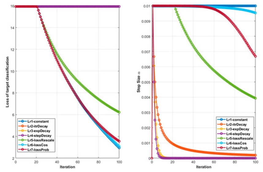
Figure 8. An illustrative sample that failed to transition to the designated target class within the 100-iteration threshold (configured with a primary step size of 0.01, moving from an initial class of 1 to a destination class of 3). The primary vertical axis tracks the progression of the target classification loss, while the secondary vertical axis monitors the reduction in step size.
Another challenging image case involving a non-targeted adversarial search is evaluated via its loss and step-reduction trajectories in Figure 9. Mirroring the previous scenario, the baseline classification loss showed no change when the step magnitude declined too aggressively (as seen with the 2nd, 3rd, and 4th decay variants). In contrast, the baseline loss began an upward trajectory following the 30th iteration when executing both the constant step size and the loss-modulated algorithms. In comparison with the targeted adversarial search sequence, the fifth approach (loss scaling function) yields tighter step intervals and minimizes the required distortion (Figure 5). Throughout the non-targeted optimization pathway, the seventh technique (original class probability) exhibits a steeper decline than the alternative loss-tracking frameworks, which results in minor total distortion (Figure 7). Consequently, because the step size drops under the trigonometric function are less abrupt than competing variants (Figure 9), it subsequently generated higher total perturbation values.
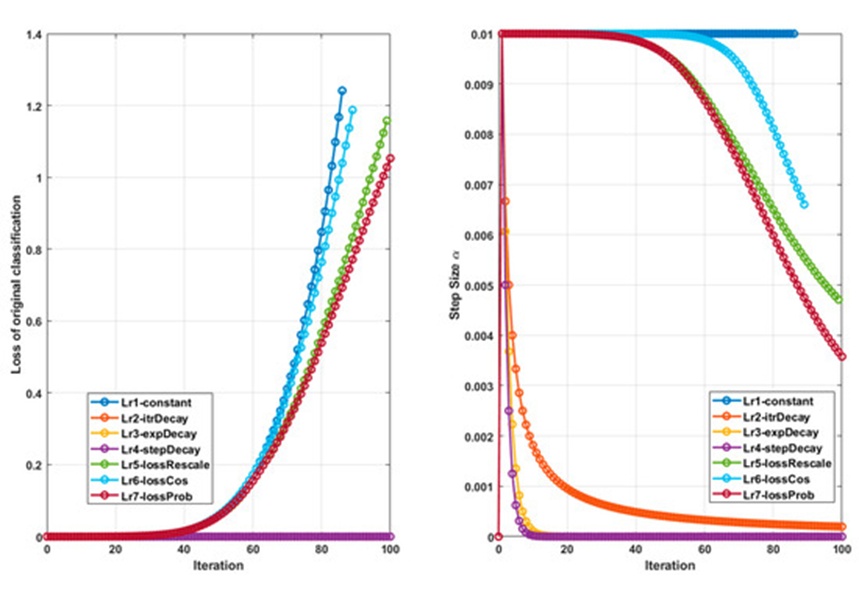
Figure 9. A resilient sample that resisted non-targeted misclassification within the 100-iteration window (with a primary step size of 0.01 and an initial class of 3; only the 1st constant, 5th loss scaling, and 6th trigonometric variants successfully resolved at 86, 99, and 89 iterations, respectively). The primary vertical axis illustrates the behavior of the baseline classification loss, and the secondary vertical axis displays the diminishing step size.
While utilizing the baseline classification probability to downscale the step magnitude proves effective, certain operational vulnerabilities complicate its dependability, particularly during a targeted adversarial exploit. Unlike the target classification loss metric, which generally exhibits a smooth, monotonic decrease throughout a targeted attack, the baseline probability does not always present a steady decay profile. Instead, its trajectory can resemble a jagged polyline or drop precipitously when an intermediate, third classification zone emerges between the baseline and targeted spaces. This vulnerability is magnified when the primary step magnitude is overly large, which elevates the likelihood of overshooting into an unintended misclassification zone rather than the designated target class. In such scenarios, the step magnitude collapses near zero, completely stalling further optimization toward the target boundary. Because of this anomaly, a higher initial step magnitude paradoxically depresses the overall success rate (96.6%) when relying on the baseline classification probability for step regulation (Figure 4).
The step-reduction algorithms uniquely influence adversarial examples that demand multiple iterations to resolve. A substantial number of instances depend solely on the primary step magnitude, as a single iteration proves sufficient to shift the network's classification (Table 4). Consequently, identifying an optimal initial step size remains critical when trying to isolate an adversarial example with minimal geometric distortion.
Table 4. Total instances where a single optimization iteration was sufficient to discover an adversarial example.
Decay Strategy | Non-Targeted Attack (𝛼₀ = 0.01) | Non-Targeted Attack (𝛼₀ = 0.1) | Non-Targeted Attack (𝛼₀ = 1) | Targeted Attack (𝛼₀ = 0.01) | Targeted Attack (𝛼₀ = 0.1) | Targeted Attack (𝛼₀ = 1) |
Constant Decay (1st) | 9 | 317 | 1050 | 10 | 453 | 2621 |
Iterative Decay (2nd) | 9 | 317 | 1050 | 10 | 453 | 2621 |
Exponential Decay (3rd) | 9 | 317 | 1050 | 10 | 453 | 2621 |
Stepwise Decay (4th) | 9 | 317 | 1050 | 10 | 453 | 2621 |
Loss-Rescaled Decay (5th) | 9 | 317 | 1050 | 10 | 453 | 2621 |
Trigonometric Loss Decay (6th) | 9 | 317 | 1050 | 10 | 447 | 2617 |
Probability-Based Loss Decay (7th) | 6 | 313 | 1050 | 6 | 434 | 2608 |
Beyond simply scaling down the primary step magnitude, several alternative algorithmic adaptations can further mitigate total adversarial distortion. For instance, adjustments can be confined to a half, a quarter, or smaller designated segments of the image canvas, or restricted to a narrower subset of pixels (Figure 10). By implementing these spatial constraints, the total quantified distortion is naturally lower than when applying perturbations uniformly across the entire image grid. For example, restricting modifications to a half or a quarter of the image space during each iteration yields a shorter L-norm distance compared to full-image modification, and isolating the adjustments to even fewer total pixels minimizes the L-norm distance further (Table 5).
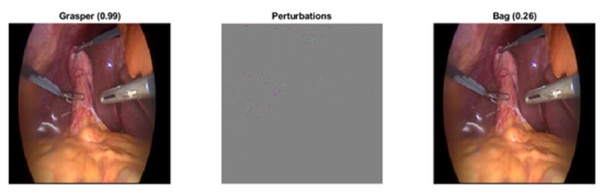
Figure 10. A non-targeted adversarial attack executed against a Grasper image (class 1) utilizing the i-FGSM framework (with a primary step size of 1 and the 6th trigonometric function regulating step reduction), where updates are confined to the top 100 highest-gradient pixels per iteration. The final adversarial pattern demonstrates that altering only 1.2% of the image canvas is sufficient to trigger a classification shift.
Table 5. The impact of varying gradient-filtering thresholds on the ultimate perturbation values required to alter the network's classification decision.
Threshold | Modify Portion | L2-Norm | L1-Norm | Iteration | Final Class | Origin Class |
0 | 99.55% | 545.89 | 15.31 × 10⁴ | 2 | 7 | 1 |
1/2 | 49.30% | 270.15 | 6.70 × 10⁴ | 2 | 4 | 1 |
1/4 | 18.65% | 181.21 | 2.82 × 10⁴ | 2 | 4 | 1 |
Top 5000 pixel | 7.71% | 127.61 | 1.25 × 10⁴ | 3 | 4 | 1 |
Top 500 pixel | 2.04% | 119.13 | 5.00 × 10³ | 12 | 4 | 1 |
Top 100 pixel | 1.18% | 158.33 | 4.08 × 10³ | 55 | 7 | 1 |
Furthermore, additional structural constraints limit the optimization's capacity to isolate the absolute minimal-distortion adversary. Our experimental setup utilized the step-adaptive iterative fast gradient sign method (i-FGSM) paired with diverse decay functions. Consequently, at each individual iteration, the magnitude of modification remains uniform across all active pixels, with only the directional vectors varying based on the gradient sign. Additionally, our loss-tracking functions treat the loss as an independent single variable detached from the core cross-entropy loss formulation J (𝜃, x, y). As a result, the calculated step size can inadvertently direct the gradient exploration into suboptimal local minima. Incorporating alternative optimization strategies capable of establishing independent, pixel-wise adaptive step sizes could greatly assist in finding tighter adversarial boundaries. Implementing high-dimensional, adaptive step-regulation frameworks established in machine learning literature [32] could allow for highly precise, pixel-level manipulation. Ultimately, the high-dimensional input and parameter spaces inherent to CNN architectures continue to pose a significant challenge for algorithms attempting to isolate the global minimum perturbation needed to alter an image's classification. However, while this step-adaptive i-FGSM was evaluated using Resnet-50, the methodology is fully transferable to alternative CNN model designs.
This study introduced a step-adaptive iterative fast gradient sign method designed for generating adversarial examples. The integrated loss-tracking functions deliver a more stable optimization path and achieve lower distortion compared to the standard, constant-step-size i-FGSM. Nevertheless, synthesizing more precise, lower-distortion adversarial examples remains possible through integration with alternative mathematical search methodologies. While adversarial training stands out as a prevalent technique for reinforcing CNN model defense, training networks on excessively distorted adversarial examples can inadvertently degrade classification performance on legitimate images. In future research, this step-adaptive iterative fast gradient sign method can be integrated into adversarial training frameworks to generate minimal-perturbation adversarial images, offering a structured pathway to analyze the trade-off dynamic balancing model robustness against general accuracy.
None
None
This work was supported by the German Federal Ministry of Research and Education (BMBF under grant CoHMed/PersonaMed KFZ 13FH5I06IA and DAAD Grant AIDE-ASD FKZ 57656657).
None
Open Access The author(s) retain copyright. This article is licensed under the Creative Commons Attribution-NonCommercial-ShareAlike 4.0 International License. It may be shared and adapted for non-commercial purposes with appropriate attribution, an indication of changes, and distribution of adaptations under the same license. Third-party material may be subject to separate terms identified in its credit line. View the license at https://creativecommons.org/licenses/by-nc-sa/4.0/.
 Transparent Intelligence Publishing