This study develops an expanded framework for extracting classification rules from neural network architectures applied to tabular data. We introduce alternative designs for learning Boolean logic operators by configuring neurons with continuous weights, including the integration of trainable NAND gates. This unified formulation ensures that distinct logical operations are trained under a singular mathematical approach, allowing developers to directly deploy established sparsity-inducing optimization routines—such as reweighted L1 regularization—to simplify the resulting network into concise rule sets. Furthermore, by utilizing De Morgan’s law, we construct an alternative network topology based on these trainable NAND components to create a NAND-NAND structure rather than the traditional AND-OR setup, both of which easily convert into discrete decision rules. Empirical evaluations show that these revised methodologies produce highly competitive decision rule models that match state-of-the-art predictive accuracy on tabular datasets.
Deploying transparent prediction models capable of offering human-interpretable rationale is vital in critical application areas like medical care and criminal sentencing, where automated determinations directly impact human lives [1]. Datasets in these specific sectors are generally structured in tables featuring inherently meaningful variables. A prominent strategy for handling tabular classification involves building decision rule sets [2-6]. Under this paradigm, the predictive model is organized in disjunctive normal form (DNF) as a collection of standalone logical constraints.
Decision rules are highly transparent by design: they consist of logical conjunctions of conditional features that must be met to trigger a positive classification. Beyond simply outputting a label, the specific activated rule within the model serves as an accessible explanation for human users. These justifications rely directly on real-world inputs, which can encompass either categorical properties (e.g., a color variable matching red, blue, or green) or numerical properties (e.g., score ≥ 100), utilizing established binary transformation techniques for processing such attributes [5, 6]. Though rule-based systems offer easily understood predictions, they frequently lag behind the predictive accuracy achieved by black-box alternatives like gradient boosting algorithms and ensemble tree methods [7, 8]. Unfortunately, understanding the inner workings of these ensemble models is exceptionally difficult for humans. This lack of transparency restricts public confidence when deploying algorithms in high-stakes fields like medical diagnosis and legal evaluation, where mistakes carry severe real-world penalties [1].
Despite their lack of transparency, deep learning pipelines are widely utilized for tabular tasks due to their high predictive capacity. At a fundamental level, deep learning uses multi-layer architectures—specifically deep neural networks with fully connected layers—to uncover sophisticated relationships hidden within data. These layers consist of interconnected computational nodes where every link weights a specific element of the underlying data. The widespread adoption of this methodology stems from its excellent generalization capabilities alongside highly optimized code libraries, like PyTorch, that greatly simplify model deployment. While fully connected layers remain the standard configuration, contemporary research is actively exploring specialized neural network designs [9, 10] optimized for tabular tasks to boost either performance or transparency.
Recently, Ref. [11] introduced an alternative framework that redefines rule learning as a neural network optimization problem. Their proposed DR-Net framework maps directly to an AND-OR logical network in disjunctive normal form (DNF), which can be converted into an interpretable set of decision rules for binary classification. Structurally, DR-Net uses a three-layer setup: the initial layer receives the inputs, the middle hidden layer uses nodes that act as trainable logical-AND operators, and the final output node runs a trainable logical-OR operator. The trainable AND nodes assemble specific rules by combining input variables, while the trainable OR node aggregates these combinations into a comprehensive rule set. As shown in [11], this setup can leverage a wide array of advanced deep learning optimization routines to match state-of-the-art classification performance while preserving the transparent benefits of classic rule models.
Even with the progress achieved by the DR-Net model, several limitations warrant deeper exploration, which this study addresses. One core problem is that the AND nodes and OR nodes in [11] rely on completely different mathematical treatments: the trainable AND components use continuous weights, whereas the trainable OR components require rounding weights strictly to 0 or 1. This operational mismatch makes it difficult to link these logic gates together inside more advanced, multi-tiered network designs. Furthermore, this discrepancy complicates the implementation of specific sparsity-inducing training methods like reweighted L1 regularization, which are critical for stripping away unnecessary connections to produce shorter, cleaner rules for tabular data tasks.
In this work, we significantly build upon the foundations laid in [11] through the following contributions:
We develop a revised formulation for trainable OR nodes that relies entirely on continuously adjusted weights, removing the necessity of weight binarization to match the implementation style of the AND node. Additionally, our new OR formulation is generalized like our AND configuration, meaning inputs can be inverted using negative weights to offer greater flexibility during optimization.
We introduce an entirely new trainable "NAND neuron" (Not AND) that operates under the exact same continuous-weight framework.
According to De Morgan’s law, an AND-OR network configuration shares logical equivalence with a NAND-NAND layout. Leveraging our trainable NAND node, we introduce an alternative network configuration named NN-Net (NAND-NAND Net) for rule extraction to serve as a counterpart to DR-Net. We also upgrade the original DR-Net framework using our updated formulations for both AND and OR nodes.
Because Boolean logic gates are now framed as trainable units using continuous weights, researchers can directly implement standard sparsity-inducing optimization routines like reweighted L1 regularization to compress the final rule sets, offering a robust alternative to the stochastic L0 regularization technique utilized in [11].
We expand our empirical validation with several new assessment routines. Specifically, we test our updated versions of DR-Net and NN-Net alongside both sparsity-inducing regularization models. We also provide new tests tracking the training dynamics to illustrate the exact effects of our sparsity-inducing mechanisms, including an analysis of training convergence and a study on how varying regularization weights changes overall model complexity.
Although tabular datasets frequently contain binary features, they typically also comprise categorical and numerical variables, which are inherently collected during data acquisition. In this study, we operate under the assumption that all inputs are binary-encoded; consequently, categorical and numerical variables must first undergo binarization via standard preprocessing techniques established in the machine learning literature. Specifically, we replicate the exact binarization methodology utilized in certain decision rule learners [5, 6], transforming all categorical variables into binary vectors through one-hot encoding. For numerical features, we apply a quantile discretization approach that accounts for the distribution of continuous values across the training set, thereby defining a collection of unique thresholds for each attribute. The original continuous value is then converted via a one-hot encoding procedure into a binary vector by comparing it against these predetermined thresholds. For instance, given age-based thresholds (e.g., age ≤ 25, age ≤ 50, age ≤ 75), a value is mapped to “1” if it is less than or equal to the threshold, and “0” otherwise. This method of binarizing continuous variables is widely adopted by decision rule induction algorithms and has demonstrated superior performance compared to direct interval discretization [5].
Following the binarization of a tabular dataset as described above, the objective of decision rule learning is to train a classifier structured as a Boolean logic function in disjunctive normal form (an OR-of-ANDs). Every logical-AND operation acts as an individual decision rule by constructing a conjunction of a subset of input features or their respective negations. A given instance satisfies a specific rule if all conditions specified within that rule are met by the instance. Conversely, the logical-OR operation aggregates these rules into a decision rule set via disjunction. The logical-OR formulation dictates that the final classification is positive if at least one rule is satisfied (i.e., the corresponding AND operation evaluates to true), whereas the final prediction is negative if no rules are met.
In formal terms, a training dataset can be mathematically represented as a collection of N data samples (𝐱𝑛,𝑦𝑛), 𝑛=1,...,𝑁, where 𝐱𝑛 denotes a vector composed of D binarized attributes 𝑥𝑛,𝑖∈{0,1}, 𝑖=1,...,𝐷, and 𝑦𝑛∈{0,1}. The discovered decision rule set can be expressed as a collection of m terms: 𝐶={𝑐1,𝑐2,...,𝑐𝑚}. We define a term c as a conjunction of k features (such as an input variable 𝑥𝑖) or their negations (such as 𝑖), where 1≤𝑘≤𝐷. If an input feature 𝑥𝑖 and its negation 𝑖 are both omitted from a term c, 𝑥𝑖 is classified as a “don’t care” feature, signifying that the value of 𝑥𝑖 (whether 0 or 1) does not influence the evaluation of term c. Based on this definition, a sample 𝐱𝑛 satisfies a term if and only if all criteria within that term are satisfied by the sample: namely, 𝑥𝑛,=1 for 𝑥𝑖 and 𝑥𝑛,𝑖=0 for 𝑖.
In this section, we outline the mathematical formulation of various Boolean logic operations interpreted as trainable neurons. Specifically, we delineate three trainable logical operators—AND, OR, and NAND (Not AND)—which serve as fundamental components for the neural network structures introduced in the subsequent section. Diverging from prior work in [11], which handled AND and OR neurons using distinct formulations, this paper introduces a unified approach for all three logic operators, structuring them as trainable neurons equipped with continuous weights and dynamic biases. We contend that this homogeneous formulation of the three logical neurons is more elegant and facilitates more uniform training across the neural networks that incorporate them.
Categorical and numerical variables are initially converted into Boolean vectors. As a result, decision rules simplify to a conjunction (or logical-AND) of these corresponding binary features. Our goal is to design a neuron that is adaptive in the following manner: given a vector of D binary variables 𝐱∈{0,1}𝐷, we aim to construct a neuron capable of being trained to compute the conjunction of a specific subset of these D variables, determined by whether their associated weights are non-zero. A weight of zero indicates that the corresponding binary feature is omitted from the conjunctive subset. Furthermore, for the binary features included in this conjunction, we intend to expand the AND operator to encompass the conjunction of either the variable 𝑥𝑖 or its negation 𝑖, dictated by whether the corresponding weight 𝑤𝑖 is positive or negative. This behavior is realized by establishing a soft mathematical formulation, followed by the application of a binary step activation function.
Specifically, using the binarized inputs 𝐱∈{0,1}𝐷 and the output y, a neuron executing a soft AND operation is formalized as:
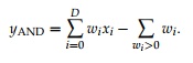 (1)
In Eq. 1, the inner product of the weights and inputs ( 𝑤𝑖𝑥𝑖) is combined with a dynamic bias term (𝑤𝑖), the value of which depends on the positive weights of the neuron. By leveraging this dynamic bias along with binarized inputs, the output range of a soft AND neuron is restricted to (−∞,0]. The output reaches exactly y = 0 if and only if the inputs align perfectly with the signs of their respective weights: inputs must equal 1 when paired with positive weights and 0 when paired with negative weights. Consequently, a soft AND neuron can be interpreted as a logical AND gate if an output of 0 is mapped to TRUE and any negative output is mapped to FALSE. Notably, similar to the role of weights in traditional neural network layers, the presence of zero-valued weights in a soft AND neuron signifies that the respective inputs have no impact on the resulting output.
However, the outputs generated by soft AND neurons cannot be propagated directly as inputs to subsequent soft AND neurons because they do not consist of binary values; thus, multi-layer architectures of purely soft neurons cannot be chained together to form a network capable of performing discrete logical operations. To ensure that soft AND neurons operate as valid logical gates during the forward pass of the neural network, binary step functions are implemented as activation functions.
The binary step activation function applied to the soft AND neurons is formulated as:
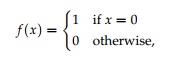 (2)
which maps an input of 0 to an output of 1, and any negative input values to 0. The activation function specified in Eq. 2 converts a soft AND neuron into a hard AND neuron that precisely executes a logical AND gate operation, given that the output evaluates to 1 if and only if all input operands are TRUE (meaning all inputs match the sign of their corresponding weights), and 0 otherwise. Because the binary step function in Eq. 2 maps continuous inputs into discrete binary integers—a transformation that is non-differentiable and incompatible with classical gradient-based optimization, we implement the straight-through estimator outlined in [12] alongside a gradient clipping mechanism. Letting 𝑖 denote the binarized activation derived from 𝑦𝑖, the gradient is computed as follows:
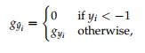 (3)
where = and = represent the gradients of the classification loss L with respect to 𝑖 and 𝑦𝑖, respectively. The restriction 𝑦𝑖<−1 is derived from the ReLU1 function, which truncates gradients for outputs that deviate by more than 1 from the maximum value. This introduces necessary non-linearity during training and empirically enhances model performance.
Similar to the trainable AND neuron detailed in the preceding section, our objective is to define an OR neuron that can be optimized to execute the disjunction (or logical-OR) over a subset of the input variables, where weights equal to zero signify the exclusion of those specific binary variables. Furthermore, mirroring our formulation of the AND neuron, we extend the OR neuron to encompass the disjunction of either a binary feature xi or its negation 𝑖, depending on whether the associated weight wi is positive or negative.
In [11], the OR neuron is structured differently. The soft OR operation in that prior study is formalized as 𝑦OR= 𝑖𝑥𝑖−𝜖, where 0<𝜖<1 represents a small value (e.g., 𝜖 = 0.5), and where 𝑖 is the binarized counterpart of the full-precision weight wi, defined such that 𝑖=0 if 𝑤𝑖≤0, and 1 otherwise. This mandatory binarization of weights diverges from the formulation of the AND neuron, which utilizes continuous weights. These distinct mathematical treatments of the two logical operators complicate their integration within multi-level neural network architectures, and also hinder the application of specific sparsity-inducing training techniques, such as the reweighted L1 regularization utilized in this study:
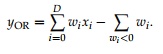 (4)
Specifically, analogously to the soft AND neuron, we formulate a soft OR neuron as follows: it resembles a soft AND neuron because it likewise computes a dot product combined with a dynamic bias, but this dynamic bias is contingent upon all negative weights of the neuron, contrasting with the positive-weight dependency in the soft AND neuron. Due to the inverted sign of the dynamic bias relative to the soft AND neuron, the output range is similarly inverted to [0,∞), where a value of 0 denotes FALSE and can only be achieved when no inputs correspond with the signs of their respective weights. While an output of 0 can be produced by both soft AND and soft OR neurons, its meaning is reversed: it signifies TRUE for soft AND neurons but FALSE for soft OR neurons.
An advantage of employing the aforementioned formulations to define soft AND and OR neurons is that these neurons remain interchangeable with classical conjunctions and disjunctions while remaining fully differentiable. The dynamic bias provides a logical interpretation for the signs of the trainable weights and the resulting output values. Specifically, the operands of the soft AND and OR operations evaluate to TRUE when the neural inputs match the signs of their corresponding weights, and the soft AND and OR neurons yield an output of 0 (signifying TRUE for AND neurons and FALSE for OR neurons) only when all operands evaluate to TRUE and FALSE, respectively. Furthermore, because the dynamic bias relies exclusively on linear calculations such as multiplication and subtraction, it is completely differentiable, which facilitates unobstructed gradient flow during backward propagation.
The soft OR neuron can be upgraded to a hard OR neuron by applying a comparable binary step activation function:
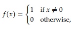 (5)
where the gradients are evaluated as:
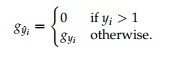 (6)
As demonstrated subsequently, these hard logic neurons serve as indispensable building blocks for the decision rules network, guaranteeing that the inferences produced by the network align identically with the extracted decision rules.
In addition to the AND and OR operations, the NAND operator can be utilized as a foundational component for the decision rule set. As detailed in the following section, stacking two layers of NAND operations is functionally equivalent to, and can be readily mapped into, an OR-of-AND configuration. Given that a NAND operation is defined as an AND operation followed by output inversion, we can formulate the soft NAND neuron by applying a negation function to the output of the soft AND neuron:
 (7)
Recall that the soft AND neuron formalized in Eq. 1 generates a continuous value restricted to (−∞,0], where an output of 0 is reachable only when all inputs match the signs of their corresponding weights. The negation function in Eq. 7 simply flips the soft AND neuron's output to fall within the range [0,∞). Because the output of the soft NAND neuron can be interpreted identically to that of the soft OR neuron, the binary step activation function defined for the soft OR neuron in Eq. 5 can be employed to convert the soft NAND neuron into a hard NAND neuron. Consequently, the soft NAND operation—comprising a soft AND operation and a negation function—coupled with the binary step activation function from Eq. 5, functions as a logical NAND gate that outputs 0 when all inputs match the signs of their respective weights, and 1 otherwise. In short, a soft NAND neuron is constructed by pairing a soft AND neuron with a negation function, while a hard NAND neuron is realized by subsequently applying a binary step activation function.
In this section, we begin by reviewing the DR-Net framework introduced in [11]. However, in this study, we substitute the original AND and OR operators with our newly proposed formulations. Additionally, we introduce a novel neural network architecture designated as a NAND-NAND net by leveraging the NAND neuron formulation, which similarly maps to a set of decision rules in disjunctive normal form (DNF) via De Morgan's laws.
As explained in [11], the decision rules network (DR-Net) is configured as a basic three-layer neural network. This setup consists of an input layer with n units, a hidden layer containing k neurons, and an output layer that terminates in a single neuron. To demonstrate the underlying principles of the DR-Net framework, Figure 1a provides a simplified toy model designed for predicting university admissions. In this scenario, the first input, designated "GPA ≥ 3.0", signifies that an applicant's high school grade point average is 3.0 or higher. The second input, "SAT ≥ 1000", establishes that the applicant scored no less than 1000 on their college entrance examination. The final two input units track whether the candidate possesses professional work experience and compelling letters of recommendation, respectively.
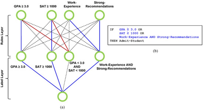
Figure 1. (a) An illustration of the DR-Net setup configured with 4 AND neurons. Positive weights leading to the AND neurons are indicated by blue lines, whereas negative weights are marked by red lines. A dashed line denotes that the linked input feature has been left out. Note that within the third rule, "NOT (GPA ≥ 3.0)" is translated to "GPA < 3.0". In the same manner, "NOT (SAT ≥ 1000)" is shown as "SAT < 1000". For the output OR neuron, a blue line indicates the rule is part of the final rule set, while a dashed line signifies its omission. (b) The network architecture maps directly onto the corresponding decision rule set displayed in the box on the right.
Each of the n input units forwards its assigned binarized value to every neuron residing in the hidden layer. This hidden tier, known as the Rules Layer, utilizes k AND neurons to carry out k logical-AND computations. The final output unit, termed the Label Layer, performs a disjunction (logical OR) across the k AND neurons from the preceding hidden layer.
Looking at the Rules Layer in Figure 1a, blue lines represent positive weights, red lines reflect negative weights, and dashed lines represent zero weights—meaning those specific inputs are omitted from the resulting rule. For instance, the first neuron in the hidden layer translates directly to the condition "GPA ≥ 3.0". For the third hidden neuron, the red connections dictate "NOT (GPA ≥ 3.0) AND NOT (SAT ≥ 1000)", an expression logically identical to the rule "GPA < 3.0 AND SAT < 1000". The final neuron represents the condition "Work Experience AND Strong Recommendations". Similarly, in the Label Layer, blue lines denote positive weights to show that a rule is included in the final set, while dashed lines signify zero weights to show a rule's exclusion. Working in tandem with the hidden layer of AND neurons, the comprehensive DR-Net setup functions as a trainable AND-OR network. This system represents a Boolean formula in DNF that translates directly into an un-ordered group of IF-THEN rules, as modeled on the right side of Figure 1b.
The fundamental departure between this study and the earlier research detailed in [11] centers on how the AND and OR neurons are defined. Both neuron types are now structured identically using continuous weights. This uniform design permits them to undergo training via distinct regularization pathways, such as the sparsity-driven regularization algorithms. Additionally, the formulation of the OR neuron has been expanded to accommodate input negation. The general definition of the OR neuron allows it to encompass the disjunction of a binary variable xi or its inverse 𝑖, dictated by whether the associated weight wi possesses a positive or negative value.
A modification of the initial diagram is presented in Figure 2. As shown in Figure 2a, a negative weight in the Label Layer is marked by a red line, signaling the negation of that specific rule. In this instance, the AND rule produced by the third hidden layer neuron is "GPA < 3.0 AND SAT < 1000". The red connection running to the output OR neuron means this entire expression is inverted. According to De Morgan's law, this inversion alters the AND rule by reversing each binarized attribute and connecting them with an OR operator, ensuring the resulting logic continues to conform to a disjunctive normal form. Specifically, the inverse of "GPA < 3.0" becomes "GPA ≥ 3.0", and the inverse of "SAT < 1000" becomes "SAT ≥ 1000". Consequently, negating "GPA < 3.0 AND SAT < 1000" yields "GPA ≥ 3.0 OR SAT ≥ 1000", which maps to the exact same decision rule set shown in Figure 2b. The rule tied to this negative weight is highlighted in red within the IF-THEN rules of Figure 2b.
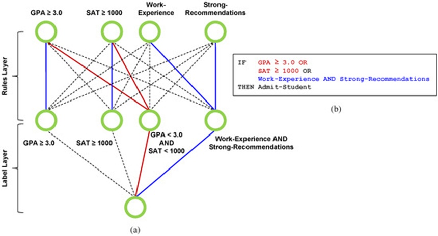
Figure 2. (a) A modified version of the example from Figure 1, where the red line leading to the output OR neuron marks the negation of the rule "GPA < 3.0 AND SAT < 1000." Applying De Morgan's law converts the negation of "GPA < 3.0 AND SAT < 1000" into "GPA ≥ 3.0 OR SAT ≥ 1000," leaving the final decision rule set unchanged. (b) The matching decision rule set is displayed on the right side.
Beyond updating the DR-Net framework with our new formulations for AND and OR neurons, we introduce an alternative decision network design known as the NAND-NAND network (NN-Net). This approach also relies on a three-layer, fully connected neural network that outputs a decision rule set in disjunctive normal form. It binarizes numerical and categorical features using the exact same strategy as DR-Net. The primary structural distinction lies in the operations performed by each tier: whereas the Rules Layer and Label Layer of DR-Net execute a collection of logical AND operators and an OR operator, respectively, NN-Net strings together two consecutive tiers of cascading NAND operators within its Rules and Label Layers.
As previously established, the DNF decision rule sets produced by DR-Net can be conceptualized as an OR-of-ANDs layout, which naturally uses multiple AND operators feeding into a singular OR operator. Mathematically, letting 𝑝𝑘,∈{𝑥𝑖,𝑖} represent the i-th predicate within the k-th rule, a decision rule set is formalized as follows:
 (8)
where ⋁ and ⋀ denote OR and AND operations, respectively. Following De Morgan's laws, the inverse of a disjunction matches the conjunction of the individual negated terms: = ⋀. As a result, the DNF statement in Eq. 8 can be restructured into two sequential levels of conjunctions:
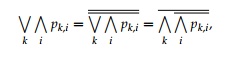 (9)
where acts as a logical-NAND (NOT-AND) operator. In other words, a NAND-of-NANDs pipeline is logically identical to an OR-of-ANDs pipeline. Consequently, NN-Net maintains the precise structural layout of DR-Net, substituting the hidden layer with n hard NAND neurons and the output layer with a single soft NAND neuron.
Though built on a different formulation, NN-Net can be deciphered using the same logic as DR-Net. That is, the hard NAND neurons in the Rules Layer of NN-Net isolate rules in the same manner as the hard AND neurons in DR-Net's Rules Layer, which are then filtered by the soft NAND neuron in the Label Layer. The logical parity between the rule translations of NN-Net and DR-Net relies on two main insights: (1) the inversions resulting from the Rules Layer NAND outputs can be decoupled and integrated into the Label Layer, and (2) in accordance with De Morgan's laws, negating the inputs of the Label Layer's NAND neuron fundamentally executes an OR operation. The first insight indicates that a series of conjunction rules can be readily derived from the Rules Layer weights of NN-Net just as they are in DR-Net. The second insight shows that interpreting the disjunction of these rules requires evaluating the weights of NN-Net's output neuron. Specifically, because of the extra input inversion inherited from the hidden layer, the NOT-NAND neuron in the Label Layer of NN-Net yields a true output if any hidden neuron generates an output that aligns with the sign of its respective weight. As a result, the Label Layer neuron aggregates the rules from the Rules Layer disjunctively, where positive and negative weights demand positive and negative rule associations, respectively, while zero-valued weights eliminate the rules entirely.
The neural network frameworks introduced in this study—namely DR-Net and NN-Net—present a novel methodology for extracting decision rule sets by utilizing stochastic gradient descent as an optimization framework. A defining trait of these networks is that zero-valued weights within the Rules Layer and Label Layer signify the complete exclusion of their corresponding input features and rules, respectively. Consequently, maximizing the sparsity within these two layers minimizes the number of conditions contained in the rule set while simultaneously purging redundant rules. However, achieving an exact zero weight remains a structural challenge during conventional network training, given that the widely implemented L1 regularization does not explicitly penalize non-zero parameters.
To directly minimize the structural complexity of the extracted rule set, prior research [11] introduced only a single sparsity-inducing mechanism based on the recently proposed L0 regularization. In this study, the newly developed uniform definitions for AND, OR, and NAND neurons permit more adaptable pruning techniques to be integrated into our networks without requiring custom modifications. To realize a substantial number of exact zero weights, we explore the integration of two distinct sparsity-driven mechanisms into the training workflow: (1) the recently introduced L0 regularization technique, which attaches trainable mask variables to all network weights, and (2) the reweighted L1 regularization approach [13], which forces weights possessing small absolute values toward zero by employing a log-sum penalty function.
In particular, this sparsity-promoting regularization is applied across both the Rules Layer and the Label Layer in the following manner:
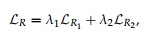 (10)
where the respective terms represent the regularization penalty functions for the Rules Layer and the Label Layer, while 𝜆1 and 𝜆2 denote the corresponding regularization coefficients that balance classification accuracy against rule set complexity. Conceptually, larger values of 𝜆1 and 𝜆2 yield a lower number of conditions per rule and a reduced count of rules, respectively. By incorporating the regularization methods defined in Eq. 10, the comprehensive loss function optimized during training can be formulated as follows:
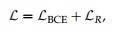 (11)
where ℒBCE represents the binary cross-entropy loss.
Following the L0 regularization framework for enforcing network sparsity outlined in [14], each individual weight is linked to a binary random variable 𝑧𝑖∈0,1 that dictates its retention or elimination. This allows each weight wi to be expressed as the product of an adjusted weight value 𝑖 and its associated binary random variable zi:
 (12)
Assuming that each zi adheres to a Bernoulli distribution governed by the parameter 𝜋𝑖, which denotes the probability of zi equaling 1, i.e., (𝑧𝑖|𝜋𝑖)=Bern(𝜋𝑖), Ref. [14] implements L0 regularization by incorporating all 𝜋𝑖 parameters into the objective loss function. This penalizes the likelihood of the masks being active (equal to 1), thereby enhancing overall network sparsity. This regularization scheme is straightforwardly integrated into both DR-Net and NN-Net by replacing all standard weights with the product of their respective mask variables.
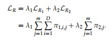
We define 𝜋1,𝑖,𝑗 and 𝜋2,𝑗 as the penalties for the non-zero mask variables associated with the neurons in the Rules Layer and the output neuron in the Label Layer, respectively, where 𝑖=1,2,⋯,𝐷 denotes the feature index and 𝑗=1,2,⋯,𝑚 represents the index of the j-th neuron. Consequently, the regularization loss ℒ𝑅 referenced in Eqs. 10 and 11 can be explicitly detailed as follows:
 (13)
Alternatively, the reweighted L1 regularization strategy introduced in [13] promotes both absolute zero weights and weights with minimal magnitudes. Specifically, this regularization method penalizes weights with smaller absolute values to drive them toward zero at an accelerated rate, thereby generating a higher concentration of weights at or near zero. Furthermore, we integrate a pruning technique [15] to eliminate weights whose absolute values fall below a designated threshold. Remaining weights near this threshold tend to be minor, making them more susceptible to exclusion from logic operations. In particular, reweighted L1 minimization is realized by applying a log-sum penalty term log(∥𝑊∥1+𝜖) across both operational layers. As a result, the reweighted L1 regularization loss ℒ𝑅 is formulated as follows:
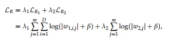 (14)
where 𝑤1,𝑖,𝑗 and 𝑤2,𝑗 correspond to the weights of the Rules Layer neurons and the Label Layer output neuron, respectively, while 𝛽>0 represents a small constant introduced to guarantee numerical stability (e.g., 𝛽=0.01).
In this section, we assess the performance of DR-Net and NN-Net integrated with the two sparsity-promoting approaches: DR-Net using L0 regularization (DR-Net-L0), DR-Net using reweighted L1 regularization (DR-Net-RE), NN-Net using L0 regularization (NN-Net-L0), and NN-Net using reweighted L1 regularization (NN-Net-RE). For each of these four variants, we trace the network convergence during training, evaluate the capacity of the sparsity-promoting mechanisms to minimize rule set complexity, verify the high predictive capability of the proposed DR-Net and NN-Net architectures, and execute comparative analyses against contemporary state-of-the-art rule learning techniques regarding the trade-off between accuracy and complexity.
The empirical assessments were conducted using four public tabular learning datasets, each containing a training set of more than 10,000 instances. The first two datasets, obtained from the UCI Machine Learning Repository [16], are the Adult Census (adult) and the MAGIC Gamma Telescope (magic) datasets. These benchmarks have frequently appeared in recent literature focusing on decision rule learning [5, 6, 17]. The remaining two benchmarks are the FICO HELOC dataset (heloc) [18] and the home price prediction dataset (house) [19]. Following the methodologies established in prior comparative works [5, 6], categorical and continuous attributes are initially converted to binary features via standard encoding techniques.
The experimental outcomes generally quantify the test accuracy alongside the structural complexities of the generated decision rule sets. We track three distinct metrics to capture various structural attributes of the decision rule models: the number of rules, the rule complexity, and the overall model complexity. Here, model complexity is quantified as the sum of the total number of rules and the cumulative number of conditions across the entire rule set. Rule complexity is defined as the mean number of conditions contained within each individual rule of the model.
Except where noted otherwise, training for both DR-Net and NN-Net was performed over 2000 epochs utilizing the Adam optimizer with a constant learning rate of 10^{-2} and zero weight decay throughout all trials. For uniformity, the batch size was set to 400, neuron weights within the Rules Layer were initialized via a uniform distribution spanning 0 to 1, and the weights of the output neuron in the Label Layer were initialized uniformly to 1. For the implementation of L0 regularization, hyper-parameters were aligned with those recommended in [14]. For the reweighted L1 regularization framework, the threshold for pruning was designated as one-tenth of the layer's standard deviation, and \beta was set to 0.01.
We begin by evaluating the distinct training behaviors of the four proposed variations (DR-Net-L0, DR-Net-RE, NN-Net-L0, and NN-Net-RE), followed by an investigation into the potential impacts of various hyper-parameters on the final decision rule configurations. The empirical observations in this subsection were gathered by training all four network configurations on the adult dataset, where each network's Rules Layer was initialized with 1000 neurons to provide adequate modeling capacity.
Training Convergence and Complexity Reduction. Through this experiment, we empirically validate that the combination of dynamic bias and the binary step activation function, integrated with the modified straight-through estimator, establishes a stable training trajectory. Figure 3 illustrates the progression of four tracking metrics (training loss, training accuracy, number of rules, and rule complexity) recorded during training across all four variants as a function of the training epochs. For these trials, training was executed on the full adult dataset with regularization weights configured at 𝜆1=10−1 and 𝜆2=10−5. Note that the visualization restricts focus to the first half of the training timeline (the initial 1000 epochs); the subsequent 1000 epochs are excluded to optimize space, given that all four tracking metrics reached a stable steady state across all networks after the 1000th epoch.
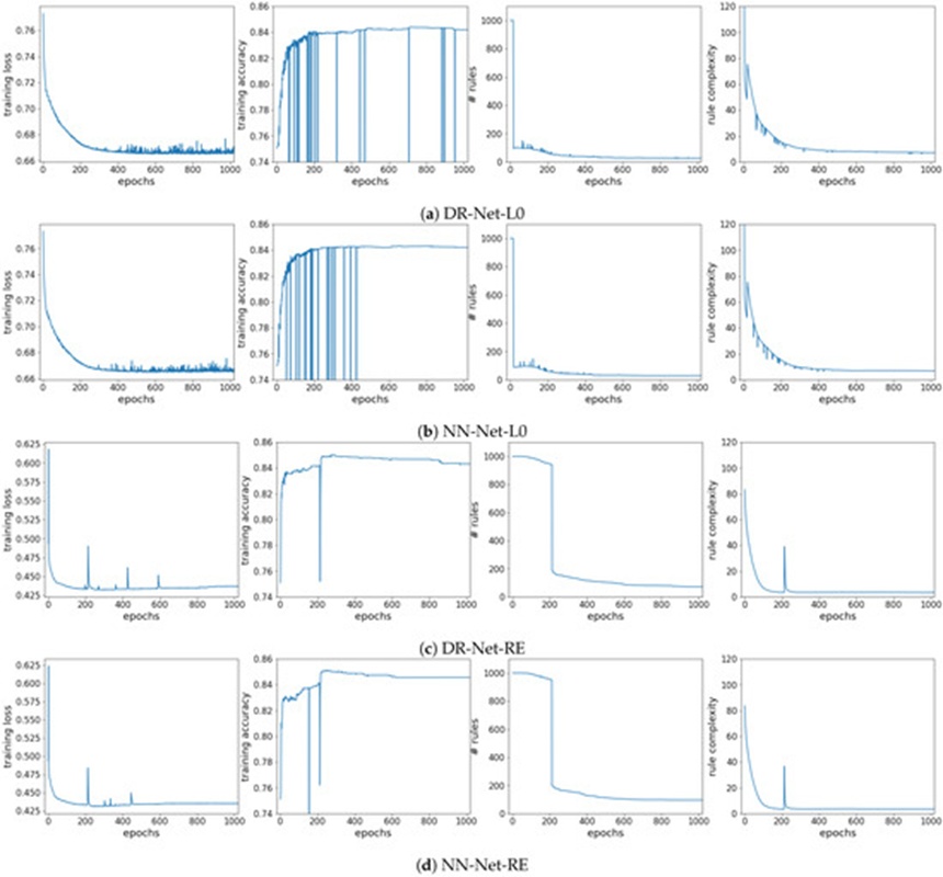
Figure 3. Training statistics (training loss, training accuracy, number of rules, and rule complexity) as functions of the number of epochs in the training process.
First, the evaluation reveals that DR-Net configurations (DR-Net-L0 and DR-Net-RE) display matching metric trajectories to their NN-Net counterparts (NN-Net-L0 and NN-Net-RE). This experimentally confirms the functional equivalence of their architectures and demonstrates that our specialized neuron formulations effectively replicate Boolean logic operations. The general direction of the curves aligns with theoretical expectations. Specifically, training losses, total rule counts, and rule complexities decrease consistently alongside epoch progression, achieving convergence at approximately epoch 400 for all variants. Concurrently, training accuracy climbs from an initial baseline of 0.75 (where all predictions default to 0) to an approximate plateau of 0.84 as training continues.
However, noticeable downward spikes occur during the training of networks utilizing L0 regularization, wherein training accuracy rapidly plummets to roughly 0.25 before recovering to its baseline level in the subsequent epoch. Minor complementary spikes and drops are also discernible in the rule count and rule complexity curves, respectively, aligning precisely with the sharp performance drops observed in the training accuracy metrics. These behavioral fluctuations during training take place when a weight within the Label Layer transitions to a negative value. Consequently, the associated rule in the Rules Layer is automatically refactored into a collection of rules where each rule contains a single inverted feature according to De Morgan’s laws. This mathematical conversion from a negated rule into multiple single-feature rules accounts for the sudden expansion in total rule count and the concurrent drop in mean rule complexity. Because nearly every data sample has an exceptionally high probability of triggering at least one of these newly expanded single-feature inverted rules, the network defaults to predicting the positive class for all inputs, precipitating the sharp drop in training accuracy. Nevertheless, the curves demonstrate that continuing optimization for just a single additional epoch readily corrects this condition. Consequently, negative weights in the Label Layer are typically absent in practice provided that all Label Layer weights are given positive initial values.
Lastly, we observe that the total number of rules undergoes a sharp reduction during the opening epochs of training for DR-Net-L0 and NN-Net-L0, as unneeded rules are identified and pruned simultaneously. A similarly sharp contraction in rule count occurs for the networks optimized with reweighted L1 regularization around epoch 200, which accounts for the temporary disruptions seen in the corresponding curves of Figures 3c, 3d.
Effects of sparsity-promoting mechanisms. The structural complexity of the derived rule sets can be modulated by selecting distinct pairs of regularization coefficients, 𝜆1 and 𝜆2. Theoretically, the Rules Layer penalty coefficient 𝜆1 governs the number of conditions active per rule (measured via rule complexity), whereas the Label Layer penalty coefficient 𝜆2 dictates the total volume of rules retained. In this experiment, we analyze the operational efficacy of the two proposed sparsity-promoting techniques by altering these regularization parameters and monitoring the corresponding changes in rule complexity and rule count. Specifically, we trained all four configurations across five distinct settings for 𝜆1 and five distinct settings for 𝜆2 using a five-fold cross-validation protocol on the adult dataset. The resulting average complexity profiles (rule complexity and number of rules) along with their standard deviations across the various regularization values 𝜆1 and 𝜆2 are displayed in Figure 4.
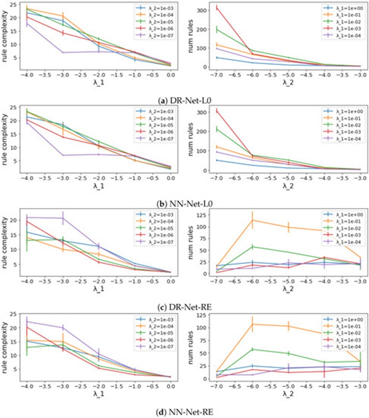
Figure 4. The relations between complexities (rule complexity and number of rules) and regularization parameters 𝜆1 and 𝜆2. All x-axes are on a log10 scale. All complexity values were averaged over five cross-validation partitions, and the vertical bars represent standard deviations.
In the left-hand column of Figure 4, each trend line charts the modification in average rule length as 𝜆1 scales upward under a fixed value of 𝜆2. Across all four variations, the average rule length drops monotonically as 𝜆1 rises from 10^{-4} to 1 (noting that the horizontal axes utilize log scales), which highlights the strong influence of the Rules Layer regularization term across all architectures. This clean mathematical relationship between rule length and 𝜆1 endows our models with a highly predictable foundation for navigating accuracy–complexity trade-offs. Similarly, the trend lines in the right-hand column of Figure 4 indicate how the total number of rules shifts in relation to 𝜆2 when 𝜆1 is held constant for a given line. The rule count decreases monotonically as 𝜆2 escalates from 10−7 to 10−3 for networks utilizing L0 regularization, whereas no clear trend emerges between rule count and 𝜆2 for configurations utilizing reweighted L1 regularization.
Thus, when contrasted with the reweighted L1 framework, models trained via L0 regularization exhibit superior capabilities for rule reduction, since a larger 𝜆2 value reliably yields a leaner rule set. Even so, the reweighted L1 regularization pipeline remains a highly effective option, because even the maximum rule counts generated by DR-Net-RE and NN-Net-RE in Figure 4 were pruned down below 125, which represents a massive structural contraction from the initial 1000-rule layout.
Next, we highlight the advantages of our proposed architectures regarding both generalization accuracy and model interpretability by benchmarking them against three prominent rule-induction frameworks: the RIPPER algorithm (RIPPER) [2], Bayesian rule set (BRS) [5], and the column generation algorithm (CG) [6]. In contrast to classical baselines, BRS and CG represent modern rule-learning developments that explicitly embed interpretability criteria directly into their training loops. We utilized open-source GitHub implementations for these three baseline approaches, with the CG codebase [20] containing minor deviations from its original text.
When executing the comparative trials against the aforementioned decision rule learning frameworks, hyper-parameter optimization was strictly limited to parameters that directly dictate rule set interpretability. Specifically, we varied the maximum allowable conditions and the maximum allowable rules for RIPPER, as these serve as the native structural constraints within its framework to restrict final model size. For BRS, we modulated the prior multiplier \kappa, which alters the likelihood of selecting rules of varying lengths, matching the protocol detailed in [6]. The official implementation [20] of the column generation algorithm (CG) [6] provides two hyper-parameters that assign explicit penalization costs for adding rules and conditions; hence, these cost parameters were optimized during training instead of the complexity bound parameter C proposed in the original paper. Finally, for DR-Net-L0, NN-Net-L0, DR-Net-RE, and NN-Net-RE, we systematically swept across various combinations of 𝜆1 and 𝜆2.
Maximizing Accuracy. To chart the upper boundaries of our models' predictive capabilities, we also benchmarked three classical machine learning techniques: classification and regression tree (CART) [21], random forest (RF) [8], and a deep neural network (DNN). We deployed the scikit-learn [22] implementations for both CART and RF, fixing the maximum tree depth to 100 to maximize generalization capacity. The DNN model consisted of six fully connected layers separated by ReLU activations, with each hidden layer containing a static pool of 50 neurons to ensure sufficient expressivity. The DNN was trained for 10,000 epochs using a batch size of 2000, a learning rate of 10−2, and a weight decay coefficient of 10−2. Because RF and DNN architectures are widely categorized as uninterpretable black boxes, they serve as top-line performance benchmarks for what non-interpretable models can extract from these datasets.
To guarantee an equitable comparison across all rule-based systems, we implemented a nested five-fold cross-validation routine to isolate the optimal hyper-parameter configuration that maximized validation accuracy for each learner on each dataset. Additionally, the hyper-parameter search spaces were deliberately bounded so that the resulting rule structures remained simple enough for human interpretation. Consequently, for DR-Net-L0, DR-Net-RE, NN-Net-L0, and NN-Net-RE, the maximum hidden units in the Rules Layer was capped at 50. The resulting test accuracy values across all datasets are compiled in Table 1. All baseline entries in Table 1 for CG, BRS, RIPPER, CART, RF, and DNN are transcribed directly from [11].
Table 1. Test accuracy based on the nested five-fold cross-validation (%, standard error in parentheses).
Model Category | Method | House | Heloc | Adult | Magic |
Interpretable Models | NN-Net-RE | 84.89 (0.46) | 70.76 (0.66) | 82.59 (0.23) | 84.14 (0.69) |
NN-Net-L0 | 86.17 (0.50) | 70.71 (0.67) | 83.13 (0.59) | 84.45 (0.51) | |
DR-Net-RE | 84.84 (0.66) | 71.05 (0.57) | 82.50 (0.68) | 84.63 (0.53) | |
DR-Net-L0 | 85.90 (0.50) | 70.07 (0.89) | 83.09 (0.51) | 84.10 (0.82) | |
DR-Net | 85.71 (0.40) | 69.71 (1.05) | 82.97 (0.51) | 84.42 (0.53) | |
CG | 83.90 (0.18) | 68.65 (3.48) | 82.67 (0.48) | 83.68 (0.87) | |
BRS | 83.04 (0.11) | 69.42 (3.72) | 79.35 (1.78) | 81.44 (0.61) | |
RIPPER | 82.47 (1.84) | 69.67 (2.09) | 81.67 (1.05) | 82.22 (0.51) | |
CART | 82.37 (0.29) | 60.61 (2.83) | 78.87 (0.12) | 80.56 (0.86) | |
Non-Interpretable Models | RF | 88.70 (0.28) | 70.30 (3.70) | 82.64 (0.49) | 86.47 (0.54) |
DNN | 88.84 (0.26) | 70.64 (3.37) | 84.33 (0.42) | 87.07 (0.71) |
As demonstrated in Table 1, across all evaluation datasets, the various formulations of DR-Net and NN-Net consistently outperform the alternative interpretable models in test accuracy across almost all test cases. Our top-performing configuration (NN-Net-L0) achieves a generalization capacity that closely trails the black-box baselines (RF and DNN), showing a performance gap of only 3%. As expected, there is no meaningful accuracy variance between the DR-Net and NN-Net variants, since both architectures are fundamentally built around identical logical properties. The metrics in Table 1 indicate that our proposed frameworks are highly competitive options for interpretable classification tasks.
Accuracy–complexity trade-off. Finally, the accuracy–complexity trade-off characteristics were mapped across all rule-induction systems, including DR-Net-L0, DR-Net-RE, NN-Net-L0, NN-Net-RE, RIPPER, BRS, and CG. Distinct accuracy–complexity coordinates were generated for each algorithm on every dataset by executing the models across an expansive range of hyper-parameter values. These sweeps were performed on all datasets, and the consolidated results, representing the average across five-fold cross-validation, are illustrated in Figures 5 and 6. For each comparative method, the coordinates connected by line segments mark the Pareto efficient frontier; any data points falling underneath these boundaries represent suboptimal models that yield either degraded accuracy or elevated complexity. All data entries in Figures 5 and 6 for CG, BRS, and RIPPER are sourced from [11].
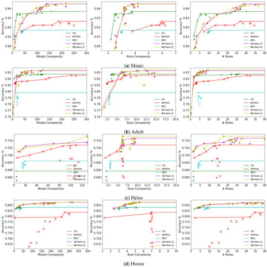
Figure 5. Accuracy–Complexity trade-offs on all datasets for DR-Net and NN-Net trained using L0 regularization. Pareto efficient points are connected by line segments.
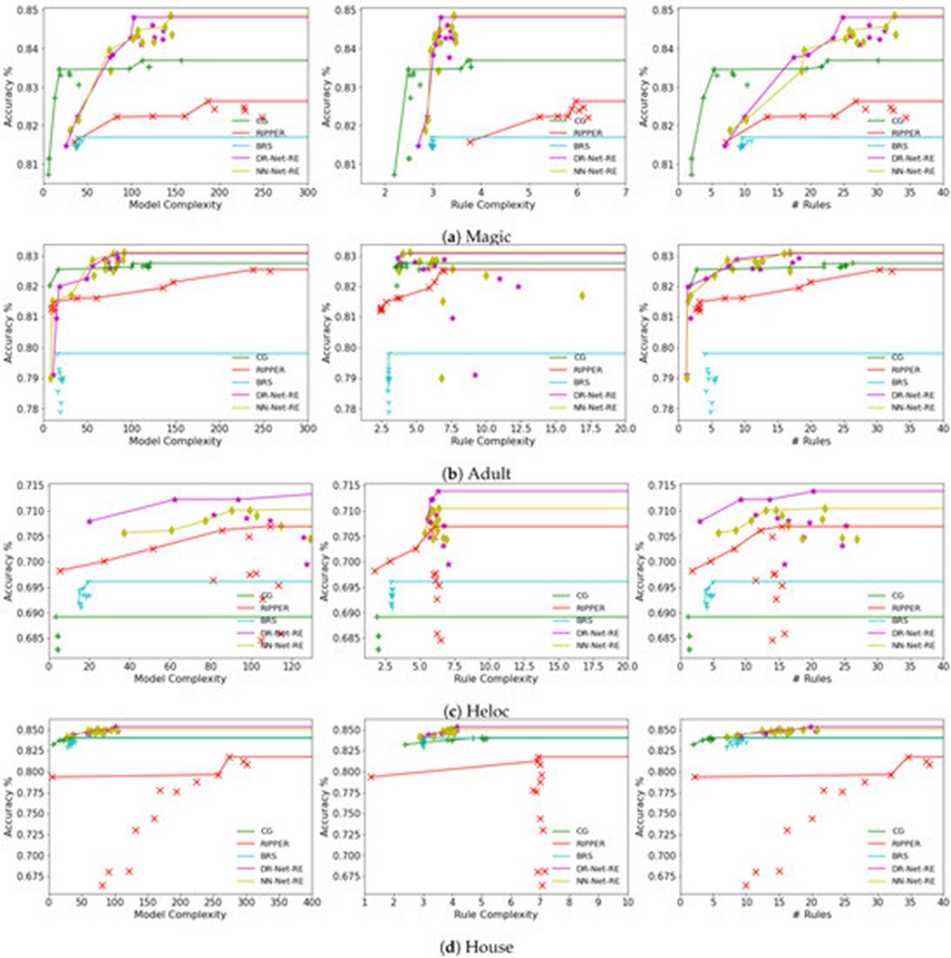
Figure 6. Accuracy–Complexity trade-offs on all datasets for DR-Net and NN-Net trained using reweighted L1 regularization. Pareto efficient points are connected by line segments.
The primary advantage of both DR-Net and NN-Net—namely, their capacity to achieve high out-of-sample accuracy while maintaining a constrained model size—is further underscored in Figures 5 and 6. On the heloc and house datasets, it is evident that all formulations of DR-Net and NN-Net thoroughly outperform competing rule learners across all three complexity metrics. This performance edge is visually confirmed by their Pareto frontiers consistently maintaining the highest positions on the plots. On the magic and adult benchmarks, the DR-Net and NN-Net models continue to exhibit superior accuracy over rival rule-induction algorithms, with this performance gap expanding significantly once model complexity, average rule length, or total rule count surpasses specific thresholds. Conversely, BRS fails to chart a clear accuracy–complexity trade-off curve, as its outputs remain tightly compressed within a very narrow boundary, an analytical observation previously identified and discussed in [6, 11]. This evaluation confirms the structural advantages of DR-Net and NN-Net over alternative rule-learning systems, driven by their ability to deliver substantially higher generalization performance with a minimal, well-regulated compromise in complexity.
The field of decision rule learning has a rich history in academic literature, historically dominated by heuristic algorithms. However, these foundational frameworks often optimized for criteria that lacked a direct alignment with either classification accuracy or structural simplicity. Notable paradigms in this category include association rule mining and subsequent classification strategies [23, 24], logical analysis methodologies [25-27], and greedy set covering techniques [2].
More recently, contemporary researchers have advanced decision rule learning algorithms by explicitlyembedding interpretability metrics directly into the algorithmic design phase. Specifically, one prominent strategy for integrating interpretability involves incorporating model complexity parameters straight into the optimization objective, facilitating the simultaneous optimization of structural simplicity alongside predictive fidelity. Certain frameworks within this domain isolate rules from a predefined pool of candidate rules, which requires executing a rule-mining algorithm as an initial preprocessing step. Examples of this paradigm include a Bayesian framework resolved approximately via simulated annealing [5] and a discrete optimization formulation tackled through local search mechanics [4]. Nevertheless, forcing the model to operate only on pre-mined rules narrows the overall search space and restricts the capacity to discover a globally optimal solution.
Alternative methodologies leverage integer programming (IP) formulations that circumvent the need for pre-mined rules entirely; however, due to the intrinsically NP-hard nature of these formulations, only approximate solutions can be recovered when dealing with large-scale datasets. For instance, the IP formulation in [6] is approximately solved by relaxing the integer constraints into a continuous linear programming problem and executing a column generation algorithm. Similarly, the framework in [3] deploys diverse optimization strategies, including block coordinate descent and alternating minimization mechanics.
Beyond decision rule sets, decision lists [28-30] and decision trees [21, 31] represent alternative paradigms for explainable, rule-based machine learning. Decision lists arrange rules into an ordered, sequential IF-THEN-ELSE hierarchy. However, this cascading design means that interpreting a targeted rule unfortunately mandates a comprehensive grasp of all preceding rule conditions, increasing the cognitive load required for human comprehension. Decision trees implicitly map rules into a hierarchical tree topology where each rule matches a distinct path from root to leaf. Nonetheless, these resulting rules are frequently overly intricate, causing decision trees to be highly susceptible to overfitting.
Spurred by the immense breakthroughs of deep neural networks in perceptual learning domains such as image recognition, researchers have recently pioneered neural network architectures tailored specifically for tabular data modeling [9, 10, 32, 33]. The methodologies introduced in [9, 10] seek to replicate the core mechanisms of gradient boosted decision trees and random forests that underpin their empirical success, achieving comparable predictive capacity using specialized neural architectures. However, much like traditional gradient boosting and random forest ensembles, these models remain uninterpretable black boxes that fail to generate human-intelligible explanations. Conversely, the frameworks presented in [32, 33] are engineered specifically to retain inherent explainability.
In this study, we extended contemporary research on decision rule learning via neural network architectures capable of robust optimization for tabular classification tasks. Specifically, we introduced alternative formulations for differentiable Boolean logic gates behaving as neurons governed by continuous weights, including a novel formulation for trainable NAND units. These structural alternatives offer a uniform treatment across diverse trainable logic neurons, allowing them to be optimized identically. Consequently, this uniformity facilitates the direct deployment of well-established sparsity-inducing neural network regularization methods, such as reweighted L1 regularization, to discover sparse network topologies that map to simplified decision rule sets, supplementing the stochastic L0 regularization pipeline previously utilized in [11]. Furthermore, we designed an alternative network layout leveraging trainable NAND neurons by applying De Morgan’s laws to establish a NAND-NAND network topology as a replacement for the conventional AND-OR formulation. Our empirical evaluations confirm that these alternative variations successfully construct precise decision rule configurations that achieve state-of-the-art predictive accuracy in tabular data applications.
Moreover, because our proposed AND, OR, and NAND neuron models share a uniform mathematical definition, layers of differing logical operators can be arbitrarily stacked in sequences distinct from the specific combinations explored in this paper. For instance, a neural network that maps directly to a Conjunctive Normal Form classifier can be straightforwardly built by cascading a layer of OR neurons into an output AND neuron. A compelling avenue for future investigation lies in exploring whether heterogeneous layers of these logical neurons can be integrated into more complex, deep configurations to unlock superior predictive capacity while preserving strict model interpretability.
None
None
This research has been supported, in part, by the National Science Foundation (NSF IIS-1956339).
None
Open Access The author(s) retain copyright. This article is licensed under the Creative Commons Attribution-NonCommercial-ShareAlike 4.0 International License. It may be shared and adapted for non-commercial purposes with appropriate attribution, an indication of changes, and distribution of adaptations under the same license. Third-party material may be subject to separate terms identified in its credit line. View the license at https://creativecommons.org/licenses/by-nc-sa/4.0/.
 Transparent Intelligence Publishing