We introduce and execute a transparent machine learning classification model designed for Explainable AI (XAI) that leverages expressive Boolean formulas. Potential domains of use include credit risk evaluation and medical diagnostics. The system utilizes a Boolean formula to establish a rule with adjustable complexity (or interpretability) for categorizing input data. This formula accommodates any operator applicable to single or multiple Boolean variables, offering superior expressivity relative to more rigid rule- and tree-based methodologies. Native local optimization methods are used to train the classifier, allowing for an efficient search of the feasible formula space. Fast Integer Linear Programming (ILP) or Quadratic Unconstrained Binary Optimization (QUBO) solvers—potentially enhanced by custom hardware or quantum systems—can identify shallow rules. By executing non-local moves that optimize across subtrees of the complete Boolean formula, we merge the expressivity and efficiency of the native local optimizer with the rapid processing capabilities of these devices. We present comprehensive numerical benchmarking data against multiple baseline models using recognized public datasets. The findings indicate that the native local rule classifier performs competitively with alternative models. Incorporating non-local moves yields comparable outcomes with a reduced number of iterations. Consequently, deploying specialized or quantum hardware could provide substantial acceleration by rapidly generating non-local moves.
The vast majority of contemporary machine learning (ML) models are highly intricate, making their internal mechanisms (which can contain billions of parameters) exceptionally challenging to comprehend and analyze. Nevertheless, explainability remains a critical or legally required component in numerous domains due to industry guidelines, particularly in high-risk sectors such as finance and healthcare. In these environments, explainable architectures deliver heightened transparency alongside two key advantages: (1) they can uncover underlying biases, which is vital for the ethical and accountable application of ML, and (2) they are often simpler to maintain and optimize over time.
Although various methodologies attempt to clarify the choices made by black-box ML systems [1], they can introduce complications such as ambiguity, incomplete fidelity, vulnerability to adversarial manipulation, and potential variance from the actual ground truth [2, 3]. Conversely, alternative strategy paths toward explainability prioritize the development of inherently interpretable ML frameworks, though sometimes at the expense of predictive performance [4-8].
In this study, we introduce an interpretable ML classification framework based on highly expressive Boolean formulas. This Boolean expression establishes a classification rule with adjustable complexity and interpretability for evaluating input features. The formula can integrate any operator applicable to one or multiple Boolean variables, including functions like And and AtLeast. This adaptability yields greater expressivity than rigid, rule-based alternatives, which can lead to enhanced accuracy and interpretability.
Over the long term, quantum computing architectures may provide computational acceleration for resolving intricate optimization challenges [9, 10]. In the shorter term, specialized classical hardware components have been engineered to accelerate ML workloads [11, 12] and optimization tasks [13, 14]. Such platforms, whether classical or quantum, generally feature a narrow domain of applicability where they offer an advantage. Furthermore, native optimization—meaning the resolution of optimization problems within their inherent representation—promises greater efficiency [15] but frequently demands a bespoke optimizer that cannot easily leverage specialized hardware. To address the explainability challenge, we design a native optimization framework that utilizes specialized hardware to rapidly resolve subproblems, thereby merging the benefits of both approaches: dedicated hardware and native optimization.
The primary contributions of this study are outlined below:
Improved and expanded Integer Linear Programming (ILP) formulations along with corresponding Quadratic Unconstrained Binary Optimization (QUBO) frameworks designed to identify depth-one rules.
A native local solver designed to determine expressive Boolean expressions.
The integration of non-local moves driven by the aforementioned ILP/QUBO frameworks (or potentially other formulations).
The core findings of this research include:
Expressive Boolean formulas deliver more compact representations than standard decision trees and conjunctive normal form (CNF) rules across a variety of scenarios.
Parameterized operators, such as AtLeast, exhibit greater expressivity than non-parameterized alternatives, such as Or.
The native local rule classifier demonstrates competitive performance relative to the established baseline models evaluated in this study.
Incorporating non-local moves produces equivalent outcomes using fewer iterations. As a result, leveraging specialized or quantum hardware architectures could yield a major speedup via the rapid generation of non-local moves.
Explainable AI (XAI) is a subfield of ML focused on clarifying or interpreting the predictions generated by machine learning systems. Generally, XAI methodologies are split into two major frameworks, which are summarized below:
Post hoc explanation of black-box models (Explainable ML)—Many of the leading ML architectures, particularly within deep learning (DL), are massive systems containing an extensive array of weights and biases, with recent networks exceeding one trillion parameters [16]. These DL configurations are inherently difficult to deconstruct. The most prevalent XAI strategies for these frameworks offer post hoc explanations of black-box determinations. These techniques are generally model-agnostic and can be deployed across arbitrarily intricate models, such as those typically found in DL.
Local explanation methods implement localized approximations across clusters of instances, such as LIME [17] and SHAP [18], or across varying feature subsets, such as MUSE [19]. These approaches frequently exhibit a lack of robustness and can often be manipulated by adversarial inputs [2, 3].
Global explanation methods seek to replicate the behavior of black-box architectures through the use of interpretable proxy models [20, 21]. These strategies profit from the straightforward collection of supplementary data generated by querying the primary black-box model. Nonetheless, ambiguity remains a challenge, as multiple distinct interpretable models might deliver an identical level of high fidelity. Furthermore, because achieving flawless fidelity is generally unfeasible, the proxy model can deviate further from the underlying ground truth than the original black-box system.
Training interpretable models (Interpretable ML)—The criteria for what renders a model interpretable varies by domain and can be highly user-dependent. Even so, many inherently interpretable architectures have been investigated. Select instances include rule lists [4], falling-rule lists [5], decision sets [6], scoring systems [7], as well as the more conventional decision trees and linear regression models. A foundation of literature also exists regarding the deployment of specific Boolean formulas as ML models. Examples include learning conjunctive/disjunctive normal form (CNF/DNF) rules through the use of a MaxSAT (Maximum Satisfiability) solver [22, 23], an ILP solver [24-26], or via linear programming (LP) relaxation methods [27].
A widespread assumption persists that interpretable models inherently deliver lower predictive accuracy than more complex, black-box alternatives. However, in many scenarios, interpretable architectures have demonstrated performance levels comparable to black-box models [28], a phenomenon frequently observed with structured datasets containing naturally meaningful features. Nonetheless, scenarios may arise where interpretable models do produce inferior results. In those instances, a reduction in accuracy might serve as a justifiable trade-off for the heightened confidence and trust provided by an understandable model.
Interpretable classifiers, including the models detailed in this study, can function as autonomous interpretable systems or can be utilized to clarify the operations of black-box models. The fundamental distinction lies in the source of the target labels: in the standalone scenario, the labels represent the absolute ground truth, whereas in the explanatory scenario, the labels correspond to the outputs generated by the black-box model.
The focus of this section is to outline the core problem framework, establish the mathematical objective functions, define the architecture of expressive Boolean formulas, and provide the justification for deploying them within the field of XAI.
We initiate our methodology by formalizing the task at hand.
Definition 1 (Rule Optimization Problem (ROP)). Given a binary feature matrix 𝑿 and a binary label vector 𝒚, the objective of the Rule Optimization Problem (ROP) is to identify the most effective rule 𝑅∗ that establishes an optimal equilibrium between the predictive accuracy score S of the rule R on the classification dataset and the structural complexity C of that rule, where complexity represents the total count of components (variables and operators) within R. Furthermore, an independent boundary parameter C' can be enforced to constrain this complexity.
From a mathematical perspective, this high-level optimization task can be formulated as:
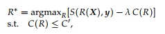 (1)
where R symbolizes any structurally valid rule, R* represents the finalized optimal rule, S denotes the evaluation score, C signifies the structural complexity, 𝑿 is the binary matrix containing the input attributes, 𝒚 is the binary vector of corresponding target labels, and 𝜆 is a real-valued scalar regulating the trade-off between classification success and model complexity. The output of this procedure is a singular classification rule. Note that this problem configuration is highly adaptable, permitting alternative architectural design choices that are elaborated upon in subsequent sections.
This problem structure handles two inherently conflicting goals: maximizing predictive success and minimizing rule complexity. The model's success is quantified via a selected evaluation metric that yields a performance score S.
Although this trade-off could be resolved using a multi-objective optimization framework, we leave that avenue for future exploration. Instead, we implement two standard strategies frequently utilized in optimization literature:
Merging distinct objectives into a unified function—We introduce a scalar parameter 𝜆 ≥ 0 that governs the relative importance allocated to structural complexity (and, consequently, to model interpretability). This 𝜆 parameter scales the precise reduction in classification score that an operator is willing to concede in order to decrease the overall rule complexity by a single unit. Generally, larger values of 𝜆 yield simpler, more compact models. We subsequently solve a single-objective optimization challenge focused on maximizing the joint objective function S - 𝜆 C, which fuses both targets into a single hybrid expression governed by the application-specific parameter 𝜆.
Imposing a strict boundary constraint on one objective—We define a maximum threshold for allowable structural complexity, denoted as C' (or maxcomplexity), and systematically alter C' to achieve the targeted configuration.
Typically, optimization formulations adopt only one of these two paradigms. We have chosen to integrate both into our framework because the scalar weighting approach offers no inherent methodology for determining an ideal 𝜆, whereas the boundary approach ensures rigorous control over rule complexity at the cost of adding an extra mathematical constraint. Generally, we favor the precise control offered by configuring C', since adding a single constraint does not introduce a prohibitive computational bottleneck. However, it is critical to note that if 𝜆 = 0, alternative rule structures that yield identical classification scores but possess different complexity metrics will evaluate to the exact same objective function value. In practical applications, the less complex rule is almost always preferred. To signal this preference to the optimization engine, we recommend maintaining 𝜆 at a small, positive, non-zero value. Precise methodologies for optimizing 𝜆 fall outside the scope of this research paper, but it is worth noting that the ideal value of 𝜆 should generally not exceed 1/C'. This is because the performance score is bounded by S ≤ 1, and we require the penalty term 𝜆 C to be scaled proportionally to S. Since 𝜆 C ≤ 𝜆 C' ≤ 1, it follows algebraically that 𝜆 ≤ 1/C'. Regardless of these guidelines, our software environment allows users to adjust C', 𝜆, both metrics simultaneously, or neither.
Without loss of generality, this research primarily utilizes balanced accuracy as the foundational performance metric. Within this setup, S corresponds to the arithmetic mean of the accuracy calculated across both distinct target classes:
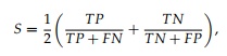 (2)
where TP represents the count of true positives, FN is the count of false negatives, FP is the count of false positives, and TN is the count of true negatives. Adjusting this setup to accommodate alternative evaluation metrics is mathematically trivial. For balanced datasets, balanced accuracy simplifies directly to standard accuracy. The primary motivation for selecting this specific metric is that real-world classification datasets frequently suffer from severe class imbalances.
A standard deployment workflow involves mapping out the performance-vs-complexity trade-off curve by altering C' or 𝜆 across a spectrum of values. This generates a sequence of candidate rules within the score–complexity space that approximate the Pareto frontier as closely as possible.
The ROP framework (detailed in Definition 1) can be evaluated across diverse rule formats. In this study, we stipulate that rules R take the form of Boolean formulas, specifically categorized as expressive Boolean formulas. An expressive Boolean formula (hereafter referred to simply as a "formula") is defined here as an arrangement of literals and operators. Literals consist of input variables fi or their corresponding negations ∼ fi. Operators represent functional operations executed on two or more literals, such as And(f0, 1, ∼ f2) and Or(∼ f0, f1). Certain operators are parameterized; for instance, \text{AtLeast2}(f0, f1, f2) evaluates to true if and only if at least two of its constituent literals are true. Operators can also be optionally negated. For simplicity of representation, we treat negation as an inherent attribute of the corresponding literal or operator rather than assigning it a dedicated \text{Not} operator node.
The integration of parameterized operators like AtLeast is inspired by the concept of highly interpretable evaluation checklists, such as a compilation of medical symptoms that indicate a specific clinical diagnosis. It is highly practical that a clinical decision would be reached using a checklist of symptoms, where a minimum threshold count must be met to trigger a positive diagnosis. Another parallel use case involves a financial institution determining whether to grant a line of credit to an applicant.
In this work, we have incorporated the operators Or, And, AtLeast, AtLeast, and Choose (Figure 1 for the comprehensive structural hierarchy of rules). The underlying definitions and implementation architecture are designed to be flexible and modular; additional operators can be introduced seamlessly (such as \text{AllEqual} or \text{Xor}), and existing ones can be omitted.
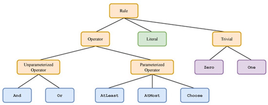
Figure 1. An overview of the logical taxonomy utilized to construct expressive Boolean expressions. The structural components are segregated into non-parameterized functions and parameterized functions. Constant baselines are available via models that output unvarying values of zero (Zero) or one (One). Inversion can be directly applied to any individual variable or functional operator.
It is highly practical to conceptualize these formulas as directed graphs (Figure 2). The terminal leaves within the graph represent the literals, which are linked via directed edges to the operator that acts upon them. To enhance visual clarity and eliminate edge crossovers, we instantiate a discrete node for each literal instance, even if that literal is referenced across multiple subsystems within the formula. Formally, this graphical structure constitutes a directed rooted tree. Computing the output of a formula for a specific set of variable inputs is achieved by initiating the evaluation at the leaf nodes, inserting the variable assignments, and sequentially applying the operator functions upwards until reaching the top of the tree structure, known as the root.
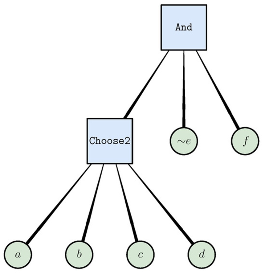
Figure 2. A visual graph of a basic expressive Boolean tree. This specific expression contains six terminal variable leaves alongside two logical operational nodes, resulting in a tree depth of two and a cumulative complexity rating of eight. The equivalent string format is And(Choose2(𝑎,𝑏,𝑐,𝑑),∼𝑒,𝑓).
We define the depth of a given formula as the longest directed path stretching from the root node to any terminal leaf (literal). As an example, the formula illustrated in Figure 2 features a depth of two. We define the structural complexity as the aggregate sum of all nodes contained within the tree, which corresponds to the cumulative count of literals and operators embedded in the formula. This exact formula possesses a complexity value of eight. This metric definition is guided by the intuitive premise that introducing supplementary literals or operators generally diminishes the baseline interpretability of a given formula. In this research, our objective centers on maximizing interpretability, which we achieve by directly minimizing structural complexity.
This section outlines the core rationale behind our research, utilizing basic examples to demonstrate how conventional decision trees and rigid rule-based models can result in excessively complicated structures when attempting to represent straightforward logical relationships.
While low-depth decision trees are generally regarded as highly interpretable and relatively efficient to train, one can easily design simple datasets that force these architectures to become exceptionally deep to maintain strong predictive accuracy. As an illustration, consider a dataset containing five binary features where an instance is classified as positive if and only if a minimum of three features are active. This straightforward relationship can be compactly expressed via the formula \text{AtLeast3}(f0, \dots, f4). However, training a standard decision tree on this data produces a sprawling architecture requiring 19 internal split nodes (as illustrated in Figure 3). Despite capturing a very simple underlying rule, the resulting decision tree becomes deep, bloated, and challenging to interpret.
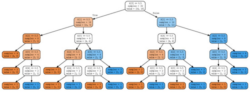
Figure 3. A diagnostic example highlighting how an intuitive classification rule generates an unwieldy decision tree graph. The mathematically ideal rule for this condition is AtLeast3(𝑓0,⋯,𝑓4), but the standard decision tree trained to mimic this data expands to 19 decision splits, sacrificing human scannability.
Furthermore, the widespread popularity of techniques that isolate optimal conjunctive normal form (CNF) or disjunctive normal form (DNF) expressions using MaxSAT engines [22, 23] or ILP frameworks [24-26] implies that such formats could serve as effective rules for classification tasks. Nonetheless, even within this paradigm, straightforward datasets can easily demand highly intricate rule expressions. Returning to the previous illustration, representing the relationship \text{AtLeast3}(f0, \dots, f4) within a strict CNF format requires an expression composed of 11 literals, 13 distinct clauses, and a total rule length of 29 (defined as the aggregate count of literals across all clauses).
Figure 4 highlights several scenarios where decision trees and CNF constraints necessitate convoluted representations for fundamentally simple logic. In this comparison, the structural complexity C of a decision tree is defined as its total number of decision nodes. Conversely, the complexity of a CNF expression is calculated conservatively as the cumulative count of all appearing literals, factoring in repetitions. For the CNF benchmarks, we evaluated alternative encoding strategies beyond those featured in the summary table, including sorting networks [29], cardinality networks [30], totalizer setups [31], modulo totalizer variants [32], and k-cardinality modulo totalizers [33]. Every single one of these alternative configurations generated more complex formulas for this data. The data reveals that decision tree configurations ("DT") are the least compact, followed by CNF formulations ("CNF"), whereas the expressive Boolean formulas proposed in this study ("Rule") offer by far the most streamlined and efficient representations for these logical conditions.
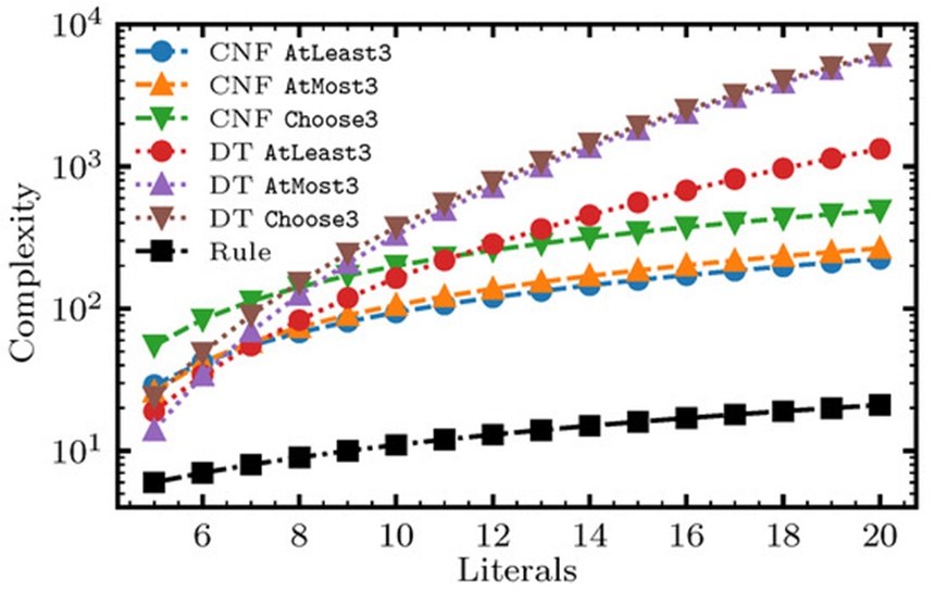
Figure 4. A comparison of the complexity required to represent rules of the form AtLeast3, AtMost3, and Choose3, varying the number of literals included under the operator. “CNF” is a CNF formula encoded via sequential counters [34], as implemented in PYSAT [35]. “DT” is a decision tree, as implemented in SCIKIT-LEARN [36]. “Rule” is an expressive Boolean formula, as defined in this paper. The complexity of a decision tree is defined as the number of decision nodes. The complexity of a CNF formula is defined as the total number of literals that appear in the CNF formula (including repetitions). The complexity of expressive Boolean formulas is defined as the total number of operators and literals (including repetitions), so in this case, it is equal to the number of literals plus one.
In this study, we propose optimizing expressive Boolean formulas by combining native local search techniques with non-local optimization procedures. In this context, the term "native" signifies that the optimization occurs directly within the problem's inherent search domain. This stands in contrast to approaches that translate the task into rigid, predefined formats such as MaxSAT, ILP, or QUBO, which can be immensely difficult (or practically impossible) and frequently demand navigating a significantly larger search space. For this problem, the natural search space consists of all valid expressive Boolean formulas. Next, the term "local" denotes the systematic navigation of this space via stochastic local search, which progresses by executing a sequence of structural modifications that impose minor updates on the active model setup [37]. Conversely, "non-local" optimization involves traversing the search domain via macro-moves that overhaul larger segments of the ongoing solution, functioning as a type of large neighborhood search [38]. The following sections detail the mechanics of our native local optimizer, introduce the concept of non-local transitions, and outline our concrete implementation.
Constructing a native local solver requires defining several primary elements: the governing constraints and search space boundaries, the initialization strategy for generating starting rules, the permitted set of local moves, the evaluation protocol for candidate rules, and the operational logic of the solver engine. Our specific design choices for these elements are detailed below, though alternative configurations could be deployed and may offer superior optimization paths.
This optimization task can be framed as an unconstrained problem by structuring the search domain such that every candidate solution generated is structurally valid. This search space remains infinite if no upper bound C' is explicitly defined. However, under these conditions, the regularizing influence of the penalty parameter 𝜆 naturally confines the solver's focus to a small subset of the total space. This occurs because the accuracy score is bounded by 0 ≤ S ≤ 1 while complexity scales as C ≥ 1. Consequently, for any designated value of 𝜆, any rule exhibiting a complexity of C > 1/𝜆 yields a negative overall objective value. Because this negative value is easily outperformed by simpler rule baselines, such overly complex expressions are effectively avoided or heavily penalized by the optimization engine.
In theory, candidate rules can encompass empty structures ("trivial rules"), individual variables, standalone operators managing two or more variables, or deeply nested hierarchies combining multiple operators and variables. In practice, trivial rules and single-variable relationships can be rapidly validated through exhaustive search, and any moderately complex dataset will require greater predictive accuracy than these basic structures can provide. Consequently, we streamline our solver by omitting these options from the primary search process. To validate this design choice and establish a clear baseline, our experimental analysis explicitly documents the performance of both the optimal single-literal (feature) rule and the optimal trivial rules (fixed constants of always one or always zero).
For parameterized operators, we restrict the search space to ensure that only logical parameter bounds are explored. Specifically, for the AtMost, AtLeast, and Choose operators, the parameter k must be non-negative and cannot exceed the aggregate count of literals assigned under that specific operator. These logical constraints are maintained inherently by structuring the initialization protocols and the proposed move sets to strictly respect these boundaries.
Initial rule structures are generated by randomly selecting between two and C' - 1 distinct literals without replacement. The sign of each literal (positive or negated) is determined via an unbiased coin flip. Following the selection of these literals, an operator type along with a structurally valid parameter (if a parameterized operator is chosen) are selected at random. These initial formulas are generated with a depth of one, while deeper structural hierarchies are explored via subsequent optimization moves.
Feasible local moves are isolated using a rejection sampling routine structured as follows. An arbitrary node (either a literal or an operator) within the active rule is selected at random. A move type is then determined by cycling through the available modification options designed for that specific node type. Next, a candidate move is randomly generated according to the chosen type. If this candidate configuration violates structural validity, it is rejected, and the loop restarts until a valid transition is identified (Algorithm 1). In practice, this process resolves rapidly, typically requiring only a handful of iterations at most.
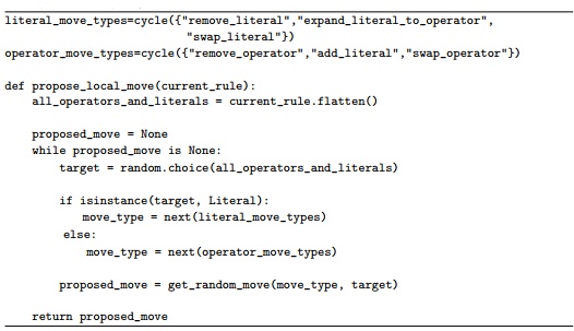
Algorithm 1. The function that proposes local moves—propose_local_move(). This function selects a node (an operator or a literal) randomly while cycling through the move types and then attempts to find a valid local move for that node and move type. The process is restarted if needed until a valid local move is found, a process that is referred to as “rejection sampling”.
The specific move types designed for literal nodes include the following actions (illustrated in Figures 5a–5c):
Remove literal—Deletes the selected literal node, provided that this removal does not leave the parent operator with fewer than two child subrules. If the parent node is a parameterized operator, its threshold parameter is automatically decreased (if required) to ensure structural validity is preserved after the literal is extracted.
Expand literal to operator—Converts a targeted literal into a full operator node, pulling a randomly selected sibling literal under the newly created operator. This step only triggers if the original parent operator retains at least one additional literal. If that parent is a parameterized operator, its threshold parameter is scaled down (if required) to remain valid following the displacement of both the target and sibling literals.
Swap literal—Substitutes the selected literal with an alternative random literal, which can either be the inverted negation of the active variable or a completely new (and potentially negated) variable not currently residing under the parent operator.
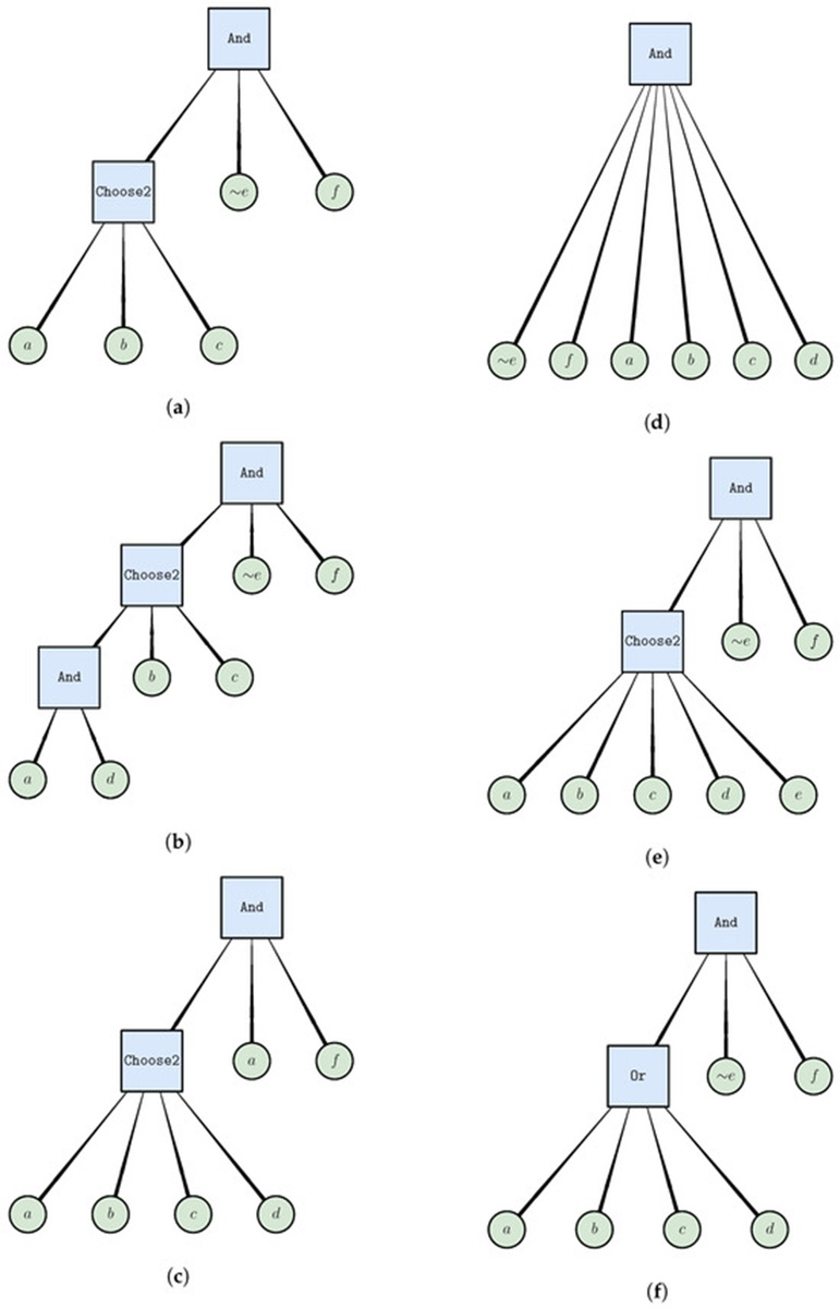
Figure 5. A visual dictionary of available local search modifications. Edits targeting individual variables are isolated in panels (a–c), while operations altering functional operators are detailed in panels (d–f). All structural shifts are executed as mutations from the baseline architecture presented in Figure 2. (a) Deletion of literal node d. (b) Transformation of literal node a into a nested And block. (c) Exchanging variable node ∼ e for feature node a. (d) Purging the Choose2 operator block. (e) Appending a new variable node e to the Choose2 cluster. (f) Reconfiguring the Choose2 block type into an Or function.
The specific move types designed for operator nodes include the following actions (illustrated in Figures 5d–5f):
Remove operator—Purges the targeted operator along with all nested operators and literals positioned beneath it. This operation is permitted only if the target operator possesses a parent node (meaning it does not function as the root of the tree) and if that parent node retains at least three subrules, ensuring the overarching formula remains structurally sound after deletion.
Add literal to operator—Appends a randomly selected literal (either positive or negated) to the target operator, provided that this specific variable is not already managed by that parent operator.
Swap operator—Exchanges the current operator for an alternative operator type selected at random, including a freshly initialized random parameter if the incoming operator requires one. This swap is executed only if the new operator type or its corresponding threshold parameter differs from the active configuration.
The quality of a given rule is determined by the mathematical framework outlined in Eq. 1, written as S - 𝜆 C. Computing this target objective necessitates evaluating the active rule across all provided input observations. This evaluation process generates a single Boolean prediction for each row in the dataset. Comparing these generated predictions against their matching ground-truth target labels yields the classification score S. In contrast, the structural complexity C depends entirely on the design framework of the rule and remains unaffected by the primary input features. Consequently, the computational overhead required to solve the objective function is heavily dominated by the rule execution step, which scales linearly relative to both the sample size and the structural rule complexity.
Computing standalone literals is immediate because the outcome corresponds directly to the state of the matching data column or its inverse complement. Evaluating operators is carried out by calculating the states of all constituent subrules and subsequently applying the operator's logic to those intermediate results. Because this calculation is typically executed across numerous observations simultaneously, it is significantly more efficient to deploy vectorized processing pipelines, which we use in our architecture. For exceptionally large datasets, this routine can also be distributed across parallel processing environments, as the rows can be evaluated independently. Furthermore, the efficiency of rule evaluation within a local optimization framework can be enhanced via memoization—specifically, caching previously resolved subrules to enable rapid lookups instead of triggering repeated computations.
The optimization workflow initiates by instantiating a fresh, randomized rule across numstarts distinct iterations. This approach injects diversification into the search landscape and is embarrassingly parallelizable. While our framework deploys a simulated annealing architecture [39], alternative stochastic local search paradigms [37] (such as greedy algorithms or tabu search variants) can be seamlessly integrated. Each distinct initialization routine starts with a baseline randomized rule and proceeds through a sequence of numiterations proposed local adjustments. Candidate moves are either accepted or rejected according to a classic Metropolis criterion, meaning that the probability of accepting a structural alteration, expressed as (Δ𝐹,)=min(1,𝑒−Δ𝐹/𝑇), is determined exclusively by the shift in the objective value Δ𝐹 and the active operational temperature T.
At the beginning of the optimization sequence, the temperature parameters are set high, causing the engine to accept the vast majority of proposed alterations to encourage broad space exploration, regardless of the specific Δ𝐹 value. This temperature parameter is systematically lowered following a geometric cooling schedule. As a result, during the final phases of an optimization run, the engine restricts its selections almost exclusively to improvements or neutral "sideways" transitions that maintain the active objective value (exploitation)—meaning moves where Δ F ≤ 0 (a sample optimization trajectory is illustrated in Figure 6).
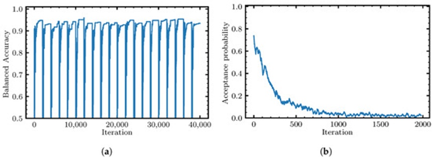
Figure 6. An optimization trajectory record tracking a native local rule session evaluated against the Breast Cancer benchmark dataset [40]. Optimization parameters are fixed at numstarts =20 and numiterations =2000, cooling through a geometric curve bounded by 0.2 down to 10−6. The transition acceptance metric tracks the running likelihood of approving a mutated candidate rule structure, computed as a moving average across active paths using a 20-step evaluation window. Graph (a) diagrams the progress of the mathematical objective calculation. Graph (b) details the corresponding trajectory of the transition acceptance metric.
The native local search architecture detailed in the previous section traverses the formula space by implementing small, incremental modifications. However, it is also practical to introduce larger, non-local transitions. Although these macro-moves demand greater computational overhead, they possess the capacity to execute substantial shifts in the objective value by broadening the operational radius of an otherwise localized search, enabling the optimization engine to break out of local minima. This section outlines methodologies for generating high-quality non-local transitions designed for compatibility with—and inspired by—quantum optimization frameworks that demonstrate acceleration relative to classical algorithms, specifically routines engineered for ILP and QUBO problems [41-44].
The fundamental principle underlying these non-local transformations is the comprehensive optimization of an entire subtree within the current formula hierarchy. Selecting an arbitrary target node (which can be either a literal or a parent operator) along with a replacement operator allows us to assign the new operator to that target position and restructure the entire underlying branch.
The targeted branch can be optimized as a depth-one configuration (comprising a single operator managing a set of terminal literals) or a depth-two configuration (featuring an operator linked to secondary operators and literals, with literals terminating the secondary branches). The optimization of this branch can be restricted to specific structural subsets, which frequently occurs when interfacing with fixed-format mathematical solvers. A classic illustration of a fixed depth-two tree structure is a DNF expression, which represents an Or operator acting upon multiple And operations. We define this branch reconfiguration as a node swap with a subtree of depth d (illustrated in Figures 7a and 7b); this research focuses primarily on configurations where d = 1.
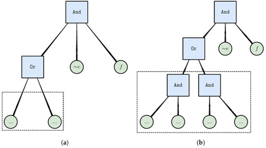
Figure 7. An architectural schematic mapping non-local transformation steps that exchange a focal node for a optimized branch structure of depth d. The provided layouts track cases where an existing operator or variable is switched out for an Or parent node backed by an optimized depth-one (a) or depth-two (b) underlying tree structure. Panel (b) provides a specific disjunctive normal form adaptation (an Or arrangement managing multiple And blocks), though alternative patterns remain supported. Both diagrams show deviations from the structural baseline established in Figure 2. The boundary region marked by the dashed border isolates the exact tree section undergoing optimization. Structural variable additions are indicated by dot placeholders, signifying that final component counts are dynamically determined.
To carry out the optimization of the subtree (T), it is necessary to identify the effective input dataset and corresponding labels for the subtree optimization task, denoted by , 𝑿′ and 𝒚′, respectively. We adopt the notation ((𝑥𝑖),𝑥𝑖) to emphasize that rule evaluation can be interpreted as first evaluating the subtree and subsequently evaluating the remaining portion of the rule using the subtree outcome. For each sample 𝑥𝑖, the rule ((𝑥𝑖),) is evaluated twice: first by assigning 𝑇(𝑥𝑖)=0 and then by assigning 𝑇(𝑥𝑖)=1. When both evaluations yield the same outcome, the result is predetermined, meaning that sample 𝑥𝑖 does not influence the score of any candidate subtree T. Conversely, when the two evaluations produce different outcomes, is assigned the value that results in a correct classification, namely such that (𝑥𝑖)=𝑦𝑖, and the associated sample is included in 𝑿′. In this situation, one of the two assignments is guaranteed to classify the sample correctly because the two distinct outcomes collectively represent all possible outputs in a binary classification setting. Consequently, the subtree score is computed exclusively using labels that are not predetermined, referred to as the effective labels. The complexity measure of the subtree (T) is evaluated using the same procedure employed for the complete rule.
To identify the non-local move, we solve an optimization problem obtained by fixing 𝑅/𝑇0 (that is, all components excluding the target node and its descendants) in Eq. 1 and eliminating constant terms, where 𝑇0 denotes the target subtree before optimization. Specifically, we obtain
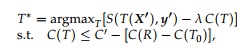 (3)
where 𝑿′ and 𝒚′ represent the input samples and effective subtree labels corresponding to the non-predetermined rows, respectively, T denotes any valid subtree, and 𝑇∗ represents the optimized subtree (i.e., the candidate non-local move).
In practical applications, it is also necessary to impose a lower bound on subtree complexity. Without such a constraint, the optimized subtree could render the overall rule invalid. Therefore, when the target node is the root, we enforce 𝚖𝚒𝚗_𝚗𝚞𝚖_𝚕𝚒𝚝𝚎𝚛𝚊𝚕𝚜=2, since the root operator must contain at least two literals. When the target node is not the root, we impose 𝚖𝚒𝚗_𝚗𝚞𝚖_𝚕𝚒𝚝𝚎𝚛𝚊𝚕𝚜=1, allowing the subtree to be replaced by a single literal whenever advantageous. For simplicity, the ILP and QUBO formulations in omit this lower-bound constraint on the number of literals; however, incorporating it is straightforward.
An additional practical concern is the need to generate non-local move proposals efficiently so that the overall solution process remains within the allocated time budget. One possible approach is to apply a short timeout. Nevertheless, the computational effort required to formulate and solve the optimization problem depends on the number of non-determined samples. When many samples are involved and the timeout is limited, the best solution obtained may exhibit low quality. To address this issue, we introduce a parameter called max_samples, which specifies the maximum number of samples permitted in the optimization problem. This parameter governs the balance between the computational effort devoted to identifying a high-quality non-local move and the speed at which such a move can be generated. Even with this restriction, obtaining the optimal solution may still require substantial computation time (for example, several minutes or longer); therefore, a short timeout is employed.
Having established the conceptual foundation of non-local transitions, we now detail how these operations are woven into the core native local optimization framework. Algorithm 2 details the procedural logic for the simulated annealing native local solver enhanced with non-local move capabilities. Because non-local transitions require higher computational overhead to resolve, they must be deployed selectively. Furthermore, these macro-moves focus heavily on exploitation rather than exploration. Consequently, introducing them during the opening phases of a simulated annealing run would fail to support broader convergence, resulting in a misallocation of computing resources.
To address this behavior, we implement a dedicated initialization phase defined as numiterationsburnin for each distinct optimization start, during which non-local moves are completely restricted. Following the completion of this burn-in window, non-local adjustments are triggered only if a designated number of successive iterations (defined as the patience threshold) pass without yielding any objective function improvements via standard local moves. A brief sample optimization run is illustrated in Figure 8, detailing the trajectory of the objective function across several distinct starts. This visualization highlights the introduction of non-local moves following the initialization phase, along with their capacity to drive clear improvements in the core objective function despite occasional rejected proposals.
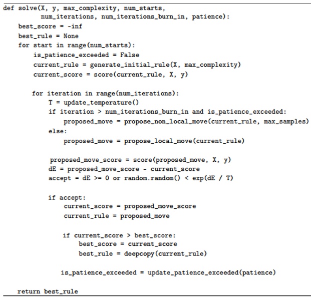
Algorithm 2. The pseudo-code for our native local solver with non-local moves. The solver executes mstartsm_{\text{starts}} starts, each with miterationsm_{\text{iterations}} iterations. In each start, a random initial rule is constructed and then a series of local (Algorithm 1) and non-local moves are proposed and accepted based on the Metropolis criterion. Non-local moves are introduced only after initial miterations_burnm_{\text{iterations\_burn}} iterations and only if there have been no improvements over a miterations_burnm_{\text{iterations\_burn}}. Both the initial rule and the proposed moves are constructed so that the current rule is always feasible and, in particular, has a complexity no higher than mcomplexitym_{\text{complexity}}. Non-local moves replace an existing literal or operator with a subtree, optimized over a randomly selected subset of the data of size msamplesm_{\text{samples}}. The solver returns the best rule found. Some details are omitted due to a lack of space
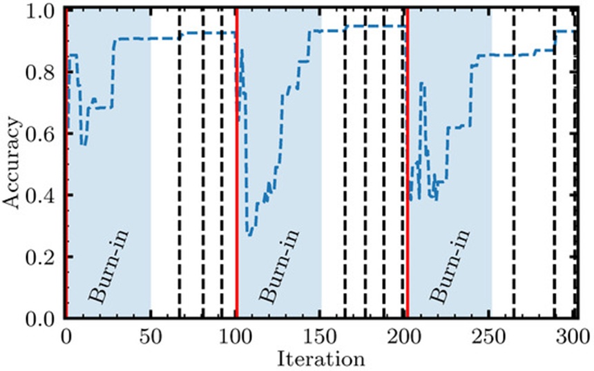
Figure 8. A tracking log detailing predictive score changes (specifically metric accuracy) throughout a brief validation test combining localized steps and macro-moves on the Breast Cancer matrix, fixing maxcomplexity =10. Engine properties are defined across numstarts =3 paths alongside numiterations =100, chilling across a geometric scale mapping 0.2 down to 10−4. Solid vertical markers in red signal the launch step of an individual optimization path. A blue container highlights the opening numiterationsburnin =50 step initialization window where macro-moves are locked out. Beyond this window, complex subtree restructurings trigger whenever local evaluations stall without accuracy improvements for a patience =10 milestone. Macro-move configurations are evaluated using compressed dataset samplings bounded by maxsamples =100, indicated by vertical dashed black lines.
This section defines the mathematical programming frameworks for identifying optimal depth-one logical expressions using an ILP or QUBO setup with varying operators configured at the root. These mathematical formulations are utilized in two distinct ways: (1) to isolate optimized depth-one logic that acts as the foundation for standalone classification architectures, and (2) to discover high-quality non-local structural shifts inside a native local solver, which systematically introduces non-local transitions.
We build upon the work of [27], which outlines the foundational methodology for structuring the search for optimal Or, And, and AtLeast relationships as linear programming challenges. The novel contributions introduced in this study encompass:
The integration of inverted (negated) input features.
The design of symmetric, even-handed mathematical formulations (unbiased with respect to positive or negative observations) alongside the integration of explicit class-balancing weights.
The structural correction of the original mathematical formulation defined for the AtLeast operator, supplemented by general extensions to accommodate AtLeast and Choose operations.
Direct algorithmic control over the accuracy-versus-complexity Pareto frontier via strict bounding constraints placed on the total count of active literals.
Subsequently, we detail the conversion of these linear programming constraints into unconstrained quadratic binary optimization (QUBO) formats. Finally, we outline how these constraints can be relaxed or softened to reduce the active search domain.
We establish our framework by noting that the logical expression y = Or(𝑓0,𝑓1) can be modeled via the following linear constraints:
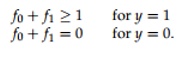 (4)
Using this relationship, we construct an optimization model designed to isolate the most compact subset of features fi to populate the Or expression to achieve flawless training classification:
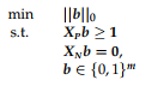 (5)
where 𝒃 represents a vector composed of binary indicator variables that signify whether a given feature is active within the classification rule 𝑏𝑖=1 if feature fi is active, and 𝑏𝑖 = 0 otherwise), 𝑿𝑷 denotes a sliced data matrix containing exclusively the observations labeled as positive (y = 1), 𝑿𝑵 denotes a sliced data matrix containing exclusively the observations labeled as negative (y = 0), and 𝟎 and 𝟏 represent column vectors composed entirely of zeros and ones, respectively.
We expand this baseline programming framework by introducing support for inverted features within the logical expression. While this capability could be achieved by manually generating inverted attributes within the raw feature space 𝑿 —which effectively doubles the dimensionality of the input matrix—it is more computationally efficient to embed the inversion logic directly within the linear formulations. To achieve this, we introduce an auxiliary vector of binary indicator variables , which details whether a given negated feature is active within the classification rule. We then replace the matrix product 𝑿𝒃→𝑿𝒃+, noting that =𝟏−𝑿 (where \boldsymbol{1} here represents a matrix filled with ones) given that any binary feature 𝑣∈{0,1} is inverted via the transformation 1 - v. Consequently, the updated expression is written as:

where||||0 matches the sum of the components of . Substituting this relationship into Eq. 5 and appending a corresponding regularization penalty for directly into the primary minimization objective yields:
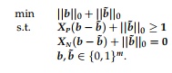 (6)
In empirical applications, achieving flawless training classification is generally unfeasible. To accommodate classification errors, we introduce a vector of binary slack variables 𝜼 that register whether a specific data observation is misclassified by the rule. When the error tracking variable linked to a given observation equals 1, the corresponding bounding constraint becomes satisfied by construction, effectively deactivating that constraint within the active optimization loop.
Accordingly, we re-engineer the primary minimization function to focus on minimizing the cumulative weighted classification errors. To regulate the structural complexity of the resulting rule, we introduce a regularization parameter alongside a strict upper-bound constraint governing the total active literal count. Finally, to handle highly skewed class distributions, we support independent weighting parameters applied to the positive and negative error terms:
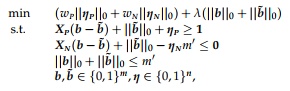 (7)
where m' (also referred to as maxnumliterals) designates the maximum number of allowable active literals, bounded such that m' ≤ m, where m represents the total count of available features; and wP and wN correspond to the positive and negative class weights, respectively. The standard configuration for these class weights is to scale them inversely proportional to the ratio of samples belonging to each respective class. In this research, we compute wP = n / (2nP) and symmetrically define wN = n / (2nN), where nP is the total count of positive samples, nN is the total count of negative samples, and n represents the total size of the dataset (n = nP + nN).
Analyzing Eq. 7 shows that when a positive data instance is misclassified (𝜂 = 1), the first tracking constraint is met by default. This occurs because the left-hand expression resolves to the sum of one plus a non-negative value, which remains strictly greater than or equal to one. Symmetrically, when a negative data row is misclassified, the second constraint is satisfied. This is because the left-hand calculation yields an evaluation bounded above by m', from which the value m' is explicitly subtracted, producing a value that is strictly non-positive. Note that this second constraint governing negative data observations was structured as an equality constraint in Eq. 6; it was transformed into an inequality constraint here to enable the error-based constraint deactivation mechanism when 𝜂 = 1.
The preceding section detailed the ILP framework structured for the Or operator. This section outlines the extension of that optimization logic to accommodate the And operator. We begin by examining why expanding beyond standalone Or expressions is necessary and outlining the mathematical symmetry connecting Or and And structures in this domain.
We highlight that De Morgan's laws confirm that every Or expression possesses a logically equivalent ∼And counterpart (and conversely, every And expression maps directly to a ∼Or structure). This structural relationship across rule distributions is visualized in Figure 9, which maps the accuracy landscapes for both single- and double-feature rule structures. The accuracy distribution for Or matches the distribution profile of ∼And (and similarly, And tracks alongside ∼Or), as mathematically anticipated. Crucially for our solver design, the accuracy profile of Or diverges substantially from the distribution profile of And, demonstrating the importance of introducing the latter operator.
Symmetrically, the accuracy profile of non-negated single-feature rules varies from the distribution profile of negated single-feature expressions, reinforcing the requirement to embed inverted features directly within the search space. As a structural note, the clear reflection symmetry visible across both plots stems from the foundational mathematical identity S(R) = 1 - S(∼ R).
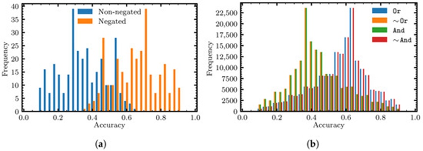
Figure 9. Accuracy score landscape for single- and double-feature rules for the full Breast Cancer dataset. Rules and respective scores are obtained by enumerating the full search space. (a) Single-feature rules. (b) Double-feature rules.
The highest-performing (optimal) rules identified for each distribution are summarized in Table 1. In this example, the top-performing And rule substantially outperforms the best Or rule, providing strong justification for its inclusion. Moreover, the importance of incorporating negated features becomes evident when the scores of the best single-feature rules are compared.
Table 1. Optimal rules for single-feature and two-feature rule configurations derived from the complete Breast Cancer dataset. “Type” denotes the rule category, “Rules” indicates the number of rules belonging to that category, “Accuracy” refers to standard classification accuracy (the evaluation metric used in this table), and “Rule” represents one of the optimal rules corresponding to the given rule category. For improved readability, feature negations are post-processed by inverting the relational operator within the associated feature expression (e.g., ∼𝑎>3→𝑎≤3)).
Rule Category | Number of Rules | Accuracy | Representative Optimal Rule |
Single Feature ((f)) | 300 | 0.647 | mean fractal dimension > 0.0552 |
Negated Single Feature ∼f | 300 | 0.914 | worst perimeter ≤ 108.9364 |
Disjunction (Or) | 179,400 | 0.931 | Or(worst concave points ≤ 0.1091, worst area ≤ 719.6364) |
Negated Disjunction (∼Or) | 179,400 | 0.944 | ∼Or(worst concave points > 0.1563, worst area > 988.6818) |
Conjunction (And) | 179,400 | 0.944 | And(worst concave points ≤ 0.1563, worst area ≤ 88.6818) |
Negated Conjunction (∼And) | 179,400 | 0.931 | ∼And(worst concave points > 0.1091, worst area > 719.6364) |
As a final motivating property, we note that as the value of maxnumliterals expands, Or rules generally exhibit a structural bias toward generating false positive errors (since accumulating supplementary features tends to pull a larger portion of outputs toward one). Conversely, And rules display an inherent bias toward generating false negative errors (since accumulating additional features forces a larger fraction of outputs toward zero). Distinct real-world deployment scenarios may favor one of these operational profiles over the other. However, both of these basic operators remain structurally rigid—a limitation that we address by introducing parameterized operators and deeper rule hierarchies optimized via the native local search engine.
To construct the ILP formulation for the And operator, we apply De Morgan's transformations. Specifically, initiating the process from the baseline model defined in Eq. 7, we switch the variable assignments such that 𝒃↔, 𝜼𝑵↔𝜼𝑷, and exchange the input data slices 𝑿𝑵↔ . This transformation yields:
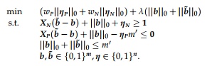 (8)
Up to this point, we have demonstrated that the process of identifying an optimal depth-one rule using root-level Or and And operators can be structured as an ILP. We now expand these models to incorporate the parameterized operators AtLeast, AtMost, and Choose. This expansion is driven by the premise that the extra parameter within these operators can offer enhanced expressivity. This flexibility may yield superior outcomes for specific datasets, particularly across certain values of maxnumliterals.
We investigate this hypothesis through an experiment where maxnumliterals is varied across its entire viable range using the Breast Cancer dataset, as illustrated in Figure 10. Within this setup, we enforce maxnumliterals=minnumliterals to isolate and reveal the authentic objective value across the full spectrum. It is readily apparent that the heightened expressivity of the parameterized operators enables them to sustain superior accuracy over the majority of the range for both training and testing datasets. Conversely, the unparameterized operators exhibit a sharp decline in performance at elevated levels of maxnumliterals. This occurs because the solver eventually exhausts the available features that can be integrated to boost the score. For parameterized operators, this bottleneck is alleviated by modulating the internal parameter accordingly.
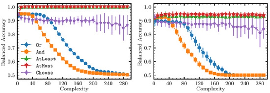
Figure 10. A comparison of the training (left) and test (right) expressivities of different operators in depth-one rules, solved via the ILP formulations. Each classifier is trained and tested on 32 stratified shuffled splits with a 70/30 split (for cross-validation) over the in-sample data (80/20 stratified split). The points correspond to the mean of the balanced accuracy and complexity over those splits. The error bars are given by the standard deviation over the balanced accuracy and complexity on the respective 32 splits for each point.
To model the AtLeast operator, we adjust Eq. 4 so that the y = AtLeastk(𝑓0,𝑓1) can be represented equivalently as:
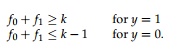 (9)
Consequently, we modify Eq. 7 to establish the ILP structure for AtLeast:
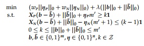 (10)
where k serves as an internal decision variable optimized directly by the solver rather than being a predetermined constant.
In a similar fashion, the AtMost operator can be formulated as:
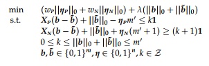 (11)
It is worth noting that any AtLeastk rule possesses an equivalent AtLeast variant of identical complexity. This counterpart can be derived by transforming k → F - k and fi →∼ fi for each feature fi within the initial rule, where F signifies the total feature count in the baseline rule. As an illustration, AtLeastk(𝑓0,𝑓1) corresponds directly to AtMost[2-k](∼𝑓0,∼𝑓1). Because of this symmetry, we anticipate comparable empirical outcomes for both AtLeast and AtMost. Nevertheless, the generated rules themselves remain distinct, and an end-user might favor one over the other based on practical interpretability.
Lastly, structuring the Choose operator presents greater difficulty due to the necessity of representing a non-equality constraint. Let us initially formulate the counterpart to the ideal Or classifier from Eq. 6 (prior to conversion into ILP form):
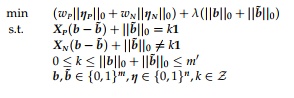 (12)
Regarding the initial constraint, any equality relation of the form a = b can be seamlessly split into a pair of inequalities, a ≤ b and a ≥ b. We have previously shown how error variables can be incorporated into inequalities within earlier models. Similarly, the non-equality constraint can be partitioned into two distinct inequalities, given that any integer-based relation of the form a \neq b translates to the disjunctive pair a ≥ b + 1 and a ≤ b - 1. While we have already outlined the method for introducing error variables to inequality constraints, these specific conditions are mutually exclusive; applying both simultaneously would render the model infeasible. To circumvent this, a well-established optimization technique for modeling either-or constraints can be utilized [45]. We introduce a vector of binary indicator variables q that dictates which of the two inequality constraints is enforced for each negative sample. This yields:
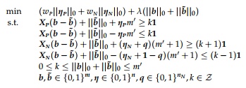 (13)
Conceptually, Choose operates as a hybrid of the AtLeast and AtMost mechanisms. Consequently, it is straightforward to observe that Eq. 13 simplifies to Eq. 10 when q = 0, and mirrors Eq. 11) when q = 1.
Our objective is to map the aforementioned ILP models onto corresponding QUBO problems, driven by the reality that a wide array of quantum hardware architectures and algorithms are fundamentally optimized for QUBO structures [42, 46-49]. We begin by outlining the conventional translation strategy [50], propose a minor refinement, and subsequently detail a structured methodology for converting an ILP into a QUBO framework.
A standard QUBO problem is generally formulated as:
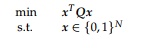 (14)
where x represents a vector comprising binary variables and Q denotes a real-valued matrix [50]. The conventional approach for embedding equality constraints, such as 𝒂𝑇𝒙=𝑏, into a QUBO involves appending a squared penalty expression (𝒂𝑇𝒙−𝑏)2, where a is a real vector, b is a real scalar, and P acts as a positive penalty multiplier.
We next outline the procedure for integrating inequality constraints, such as 𝒂𝑇𝒙≤𝑏 (without loss of generality), into the QUBO model. We begin by noting that 𝒂𝑇𝒙 is bounded from above by the sum of all positive components in a (indicated by a+) and bounded from below by the sum of all negative components in a (indicated by a-). For the inequality 𝒂𝑇𝒙 ≤ b, it is assumed that b < a+, meaning that b introduces a more restrictive bound (otherwise, the constraint serves no practical purpose). Thus, any inequality constraint can be recast into the bounded format l ≤ 𝒂𝑇𝒙 ≤ u, where l and u designate the lower and upper bounds respectively. This is the structural format utilized throughout the remainder of this section.
We can transition this inequality constraint into an equality constraint by introducing an integer slack variable bounded by 0 ≤ s ≤ u - l, which can be represented via binary encoding. Following this, the previously mentioned squaring method can be leveraged to establish the corresponding penalty term. It is crucial to highlight that this can be achieved via two distinct formulations:
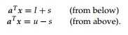 (15)
These equality equations can then be embedded by incorporating their respective penalty terms:
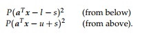 (16)
This introduces a nuanced consideration that is frequently overlooked in literature. For an exact mathematical solver, the choice between these two penalty expressions is theoretically irrelevant. However, when employing heuristic solvers, minimizing the magnitude of the problem's coefficients becomes highly advantageous. Within quantum annealing systems, the acceptable range for coefficients is constrained, and outsized values necessitate a larger scaling factor to compress the coefficients into a standardized window [51]. As this scaling factor grows, the probability increases that certain scaled coefficients will fall below the system's operational noise floor [52]. Furthermore, for many Monte Carlo approaches like simulated annealing, larger coefficients demand elevated computational temperatures to resolve, which can induce algorithmic inefficiencies.
To minimize coefficient magnitudes, we observe that the two formulations are nearly identical; they vary only by the sign preceding the slack variable s (which does not affect this analysis) and the presence of either l or u in the expression. Consequently, we advocate for selecting the penalty expression containing the bound (l or u) that possesses the smaller absolute magnitude. This choice systematically yields smaller coefficient values once the quadratic expression is expanded.
Derived from these insights, we present a streamlined protocol for translating ILP formulations into QUBO problems:
Assume a problem is structured in its canonical ILP representation:
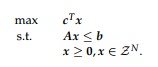 (17)
Convert the inequality conditions into equivalent equality expressions by introducing vector-valued slack variables:
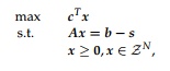 (18)
where we have adopted the "from above" setup without loss of generality.
Complete the translation to a QUBO:
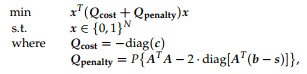 (19)
where the constant offset has been omitted, and diag(𝒄) represents a square matrix featuring the elements of c along its main diagonal.
By utilizing this structured protocol, each of the five distinct ILP frameworks can be mapped directly to its corresponding QUBO version. As a baseline example, we demonstrate this transformation using the Or formulation. We begin with Eq. 7, reproduced below for straightforward reference:
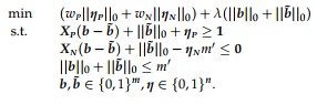 (20)
By applying the transformation protocol, we derive the following QUBO expression:
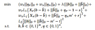 (21)
where the braces indicate a summation across the rows of the internal vector expressions, s and r denote vectors of slack variables, t represents an individual slack variable, and L1, L2 signify positive penalty multipliers. The penalty weight assigned to the maximum literal constraint must be substantially larger than the weight of the soft constraints to guarantee strict enforcement, meaning 𝐿2≫𝐿1. We refrain from explicitly writing out the constituent matrices 𝑸cost and 𝑸penalty here, as they can be easily deduced by expanding Eq. 21.
In this section, an approach is presented to diminish the total variable count within the QUBO formulation by systematically removing the error variables.
Recall that the misclassification indicator variables \eta were originally introduced to soften the constraints. This inclusion was essential for the ILP framework, where constraints would otherwise operate strictly as hard boundaries. In QUBO frameworks, however, the distinction between soft and hard constraints is determined exclusively by the magnitude of the penalty coefficients. Consequently, it is theoretically possible to eliminate these error variables from the "imperfect" formulations and instead incorporate the constraints as inherently soft, setting their associated penalty coefficients to relatively small values.
For instance, considering the Or operator, Eq. 20 can be adapted by removing the error variables from both the objective function and the constraints, classifying those specific constraints as "soft":
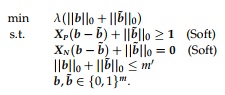 (22)
By applying the conversion protocol to each constraint and integrating the class weights, the following is obtained:
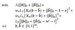 (23)
where the curly bracket notation matches the usage in Eq. 21, s represents a vector of slack variables, t is an individual slack variable, and L1 and L2 are positive penalty coefficients. As previously established, the penalty weight enforcing the maximum number of literals must be significantly larger than the weight of the soft constraints to guarantee enforcement, meaning L2 ≫L1.
The reduction in problem size achieved by relaxing these constraints is typically substantial, as detailed in the data comparison within Table 2. For the Or formulation, for instance, the addition of the \eta variables is completely bypassed for each data sample. Nonetheless, the primary mathematical savings stem from the slack variables associated with the negative data rows; because those conditions turn into exact equality constraints, the requirement for slack variables is completely avoided. Furthermore, the operational range of the slack variables for the positive data rows is narrowed, which can yield additional variable reductions. The specific variable count for each optimization model is defined by:
 (24)
Table 2. Variable requirements across alternative optimization frameworks.
Operator | ILP | without 𝜼 | with 𝜼 |
Or | 1169 | 1027 | 2879 |
And | 1169 | 1317 | 2879 |
AtLeast | 1170 | 1959 | 3097 |
AtMost | 1170 | 1959 | 3097 |
Choose | 1527 | 2673 | 3811 |
It is hypothesized that minimizing the problem size likely diminishes the time to solution (TTS). The TTS metric is conventionally computed as the product of the average duration of a single run 𝜏 and the total number of runs needed to identify an optimum within a specific confidence threshold (typically 99%), denoted as 𝑅99 :
𝜏𝑅99 [13]
Decreasing the problem size should shorten the execution time per iteration, thereby reducing \tau. Additionally, one might expect the intrinsic difficulty of the problem to decrease, leading to a smaller 𝑅99; however, this outcome is not guaranteed, as smaller optimization landscapes are generally, but not always, less complex to navigate.
The empirical outcomes of the experiment comparing the two structural setups (with vs. without 𝜂) for the Or and And operators are displayed in Figure 11. It is observed, qualitatively, that the “without 𝜂” model produces a comparable or superior accuracy–complexity profile. Furthermore, even when both configurations demonstrate equivalent performance, the computational runtime for the model without \eta is significantly shorter, occasionally by multiple orders of magnitude. This observation aligns with the preceding theoretical justifications; nonetheless, a rigorous analysis of the TTS for both frameworks is preserved for future investigations.
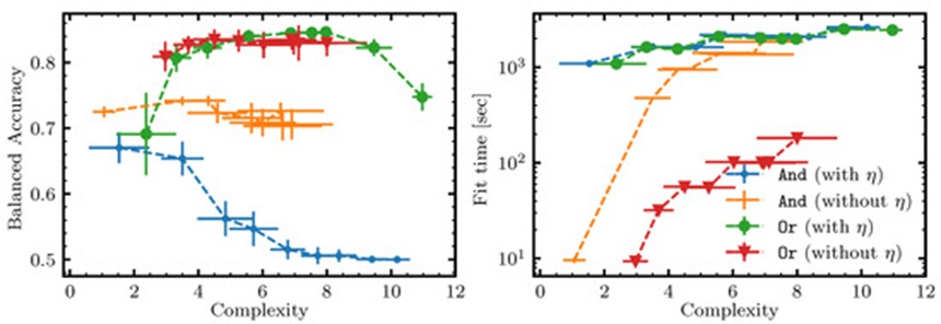
Figure 11. This multi-panel plot tracks performance accuracy alongside computational execution time for the depth-one QUBO classifier using Or and And functions, evaluating the versions built with explicit error variables versus those leveraging soft constraints (with/without 𝜂). The benchmarks utilize the Direct Marketing dataset [53]. Each distinct classifier configuration undergoes training and testing routines across 32 stratified, shuffled data splits using a 70/30 validation framework applied to the in-sample data partitions (which adhere to an 80/20 stratified split). The plotted markers indicate the average values for balanced accuracy and model complexity observed over those 32 partitions. The corresponding error bars illustrate the standard deviation for both accuracy and complexity computed across the 32 runs for each parameter configuration.
Lastly, it should be emphasized that removing the error variables introduces a structural bias into the solution space. The objective function under this configuration represents a sum of squared violations (residuals) of the sample constraints. Consequently, when evaluating two distinct solutions that share an identical score S (i.e., degenerate solutions), the system favors the solution exhibiting the lower sum of squared violations. In a sense, this bias can be considered rational, given that the preferred solution is "less incorrect" relative to the alternative possessing a larger sum of squared violations.
When constructing the Pareto frontier, the methodology requires solving a sequence of optimization tasks starting from a minimal complexity boundary 𝑚′ (i.e., max_num_literals) and incrementally raising it. Because of this process, evaluating how the variable count and the magnitude of the search space depend on m' is of significant interest. For brevity, this analysis is restricted to non-parameterized operators.
As indicated by Eq. 24, for a fixed dataset with dimensions n × m, the variable count within the QUBO models scales in a step-like manner as m' grows (Figure 12a). The total search space size for any given QUBO configuration is expressed as 2𝚗𝚞𝚖_𝚟𝚊𝚛𝚜, where num_vars is the variable count in that specific formulation. The search space size for the ILP model, which corresponds exactly to its feasible region, is substantially smaller and is defined by:
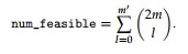 (25)
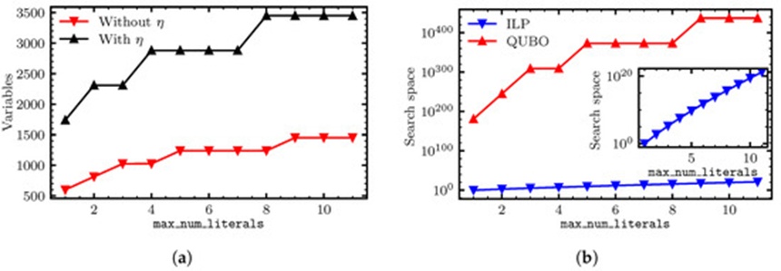
Figure 12. This pair of charts tracks how the maximum literal limit affects the underlying variable overhead and the total size of the searchable space using the Breast Cancer dataset. Plot (a) details the total variable count required by both alternative QUBO models for an Or-based rule as a function of the complexity limit m' (derived from Eq. 24). The step-like growth pattern visible in this plot is an artifact of utilizing a binary encoding system to represent the slack terms inside the inequality conditions. Plot (b) maps out the scale of the strictly feasible region (which represents the exact bounds explored by an ILP solver) against the drastically wider combination of feasible and infeasible spaces navigated by the optimized QUBO framework (constructed without \eta). The inset graphic inside plot (b) offers a highly magnified perspective focusing exclusively on the tighter ILP boundaries.
For a direct graphical comparison between the scales of the infeasible domain (QUBO) and the feasible domain (ILP), refer to Figure 12b. It is readily apparent that the domain explored by the QUBO formulations is vastly larger than the feasible region, which places the QUBO solver at a disadvantage. For instance, when \text{max\num\literals} \approx 10, the QUBO search space outscales the ILP counterpart by over 400 orders of magnitude. This divergence partly justifies utilizing the QUBO framework as a localized subproblem solver, as detailed later in this study, rather than applying it to resolve the global optimization task. When handling smaller subproblems, the scale discrepancy between the feasible and infeasible spaces is minimized and may be successfully managed by a high-performance QUBO solver.
Furthermore, a close inspection of the constraints reveals that transitioning from one feasible solution to an alternative feasible solution requires toggling multiple bits simultaneously. This indicates that the search space is characterized by isolated feasible solutions, each enveloped by a multitude of infeasible configurations featuring higher objective costs—resembling islands scattered across an ocean. This structural landscape is characteristic of constrained QUBO models. Under these circumstances, we anticipate that a localized bit-flip optimizer, such as single bit-flip simulated annealing, would face significant operational obstacles. Conversely, this specific landscape should theoretically favor quantum optimization frameworks (including quantum annealing), because the geometric barriers separating the feasible configurations are narrow, rendering them highly susceptible to quantum tunneling mechanisms [54].
This section outlines the core research questions driving our investigation, delineates the experimental configuration established for the numerical analyses, and presents a critical evaluation of the resulting empirical data.
To systematically appraise the efficacy and practical value of our proposed methodology, we address the following core research questions (RQ):
RQ1. How does each distinct optimization methodology perform relative to the Pareto frontier when mapping balanced accuracy against model complexity?
RQ2. Does the introduction of data sampling effectively facilitate scalability when processing exceptionally large datasets?
RQ3. Do non-local optimization moves offer distinct operational benefits compared to exclusively local modifications, and what specific scenarios trigger these advantages?
Datasets
The structural profiles of the binary classification datasets selected for our numerical experiments are detailed in Table 3. We deliberately compiled a suite of benchmarks exhibiting highly diverse properties. Specifically, the data volume spans from a minimal baseline of 195 instances to an expansive scale of approximately 1.3 × 10⁵ observations, while the post-processed binary feature counts range between 67 and 300 variables.
Table 3. Structural characteristics of the experimental benchmarking datasets.
Dataset | Reference | Majority Class Proportion | Binarized Features | Original Features | Number of Records |
Airline Customer Satisfaction | 0.55 | 119 | 22 | 129,487 | |
Breast Cancer Dataset | 0.63 | 300 | 30 | 569 | |
Credit Card Default Dataset | 0.78 | 185 | 23 | 30,000 | |
Credit Risk Dataset | 0.70 | 92 | 20 | 1000 | |
Customer Churn Dataset | 0.73 | 67 | 19 | 7043 | |
Direct Marketing Dataset | 0.89 | 124 | 20 | 41,188 | |
Home Equity Default Dataset | 0.80 | 93 | 12 | 3364 | |
Online Shoppers’ Intentions Dataset | 0.85 | 104 | 17 | 12,330 | |
Parkinson’s Dataset | 0.75 | 217 | 22 | 195 |
Table 3 Explanation: "Rows" denotes the total volume of complete data observations remaining after removing entries with missing values. "Features" indicates the baseline count of attributes originally provided in the dataset. "Binarized" tracks the ultimate number of distinct boolean attributes generated after executing the preprocessing pipeline. "Majority" quantifies the proportional share of data rows corresponding to the dominant class label, and "Ref." links to the authoritative source or publication for each dataset.
A subset of the source datasets contained observations with missing attributes, which were filtered out before execution. Specifically, we omitted 393 instances from the Airline Customer Satisfaction dataset, 11 instances from the Customer Churn dataset, and 2596 instances from the Home Equity Default dataset. While the data loss was minor for the first two repositories, filtering the Home Equity Default dataset removed roughly 44% of its original observations.
Constructing Boolean logic rules requires all incoming variables to be strictly binary. Consequently, any features not initially formatted as boolean were subjected to a binarization process; naturally, pre-existing binary features were preserved without modification. Categorical variables and low-cardinality numerical variables were mapped using standard one-hot encoding. For continuous or high-cardinality numerical attributes, numerous discretization strategies exist—such as equal-frequency binning, equal-width intervals, or partitions designed to optimize information gain [62]. We recognize that the selected discretization paradigm can substantially sway downstream machine learning performance, though a deeper investigation into this choice is reserved for future research.
For this study, binarization was executed by first partitioning numerical features into discrete bins and subsequently transforming them via one-hot encoding. The bin boundary locations were established by computing numbins quantiles for each targeted attribute. Each individual quantile defined an "upward" binary variable spanning from that specific quantile boundary to positive infinity. Because our classification models natively evaluate both true and inverted features, the reciprocal "downward" intervals were automatically integrated via these negated feature counterparts. Throughout all benchmarking operations, we maintained a fixed resolution of numbins = 10.
Our computational evaluations incorporated a diverse array of predictive models. First, we established the following baseline frameworks:
Most frequent: A trivial baseline model that uniformly predicts the majority class label present in the training partition. This model fundamentally yields a static balanced accuracy score of exactly 0.5. To preserve clarity and eliminate visual clutter, we omitted this baseline from our performance plots, treating it merely as an absolute lower bound that was effortlessly outstripped by all alternative models.
Single feature: A localized model whose structural complexity is restricted to a solitary feature rule. During the training phase, the optimal rule is determined by exhaustively auditing every individual feature and its corresponding negation across the entire available set.
Decision tree: A conventional decision tree model utilized via the scikit-learn framework [36], configured with the property classweight = "balanced". Because decision trees naturally handle non-binary continuous features, we also documented the performance achieved by training this model directly on the raw, unbinarized source data. We incrementally adjusted the maxdepth parameter to govern the architectural complexity of the tree, measuring its final complexity by counting its total split nodes.
The depth-one mathematical programming variants evaluated consist of:
ILP rule: A configuration that directly solves the exact ILP models to produce a depth-one rule around a designated root operator. This model was executed via FICO Xpress (version 9.0.1) under a strict runtime ceiling of one hour. To prevent computational overruns, a maximum cap of 3000 data samples was enforced for any given cross-validation partition.
QUBO rule: A configuration that computes solutions for the quadratic formulations to yield a depth-one rule centered on a given root operator. This model was executed using the simulated annealing heuristics provided by dwave-neal, utilizing the parameters numreads = 100 and numsweeps = 2000. Similar to the ILP setup, the data volume per cross-validation slice was restricted to a maximum of 3000 instances. Because its empirical accuracy scores were consistently inferior to—and mathematically bounded by—the ILP outcomes, these results were omitted from the primary visualizations to maintain clarity (though representative QUBO trajectories are visible in Figure 11). As analyzed, this performance deficit stems from the fact that dwave-neal utilizes a single-bit-flip optimizer, whereas shifting between valid solutions in our specialized QUBO formulations requires flipping multiple variables simultaneously.
Finally, we analyzed the following native local search heuristic algorithms:
SA native local rule: The specialized local-search simulated annealing classifier outlined in Section 4.5, executing with hyperparameters numstarts = 20 and numiterations = 2000. The cooling profile follows a strict geometric progression descending from an initial temperature of 0.2 down to a terminal floor of 10−6.
SA native non-local rule: An advanced iteration of the native simulated annealing classifier that incorporates non-local optimization trajectories accelerated by an embedded ILP solver. This framework shares identical baseline parameters with the standard local search engine. Additionally, it allocates the first third of its operational budget as a structural burn-in window, utilizing settings of patience = 10 and maxsamples = 100, while restricting the internal ILP subproblem solver to a maximum timeout of one second per call.
Each underlying dataset was initially segregated into an in-sample developmental partition and an out-of-sample evaluation block via a stratified 80/20 partition. The in-sample collection was subsequently randomized and partitioned 32 times (unless specified otherwise for targeted experiments) into training and validation pairs using a stratified 70/30 split. All experimental benchmarks were carried out within the Amazon EC2 ecosystem, leveraging c5a.16xlarge computing instances equipped with 64 vCPUs and 128 GiB of system memory. Cross-validation trajectories for each distinct model and dataset combination were generally processed concurrently across the 32 data splits using parallel processes on a single computing instance.
Hyperparameter tuning was kept intentionally minimal. It is highly probable that the baseline performance metrics documented here could be expanded through rigorous parameter optimization, though such fine-tuning fell outside the immediate scope of this research. Furthermore, adopting advanced mathematical programming methodologies, such as column generation routines, could substantially boost the efficiency of the ILP solvers. Lastly, note that a regularization weight of 𝜆 = 0 was applied uniformly across all numerical trials to streamline the comparative analysis.
Pareto frontier (RQ1)—For each dataset and individual classifier, we detail the mean values alongside the standard deviations for model complexity and balanced accuracy across the training and testing data splits. Because certain classifiers function without parameters, they are plotted as single coordinates for each dataset (specifically, the single-feature baseline and the most frequent label baseline). To generate the decision tree outcomes, the maxdepth configuration was modified across a diverse spectrum of settings. For the depth-one QUBO and ILP models, performance statistics were compiled by shifting the maxnumliterals constraint through a sequence of values. Lastly, the outcomes for the native local optimizers were produced by sweeping the maxcomplexity parameter over an array of limits. The decision tree was additionally evaluated directly on the raw features without utilizing a data binarizer, which is indicated in the results by the attached suffix “(NB)”.
Across the entire collection of datasets, excluding the three smallest instances containing fewer than 1,000 samples, the performance metrics on the training and testing sets are nearly identical. On account of this uniformity, we report both training and testing metrics for the smaller classification tasks, but restrict the reporting to testing metrics for the larger datasets. This close alignment between training and test results is likely driven by the design of our classifiers, which are heavily regularized through the binarization pipeline and their restricted structural complexity. Consequently, they appear highly resilient against overfitting the data, provided the training volume is not critically small.
The training and testing trajectories for the three smallest problem domains are illustrated in Figure 13, whereas Figure 14 details the isolated testing metrics for the six remaining larger datasets. Finally, a selection of representative decision rules extracted by the native local optimizer across the various domains is cataloged in Table 4.
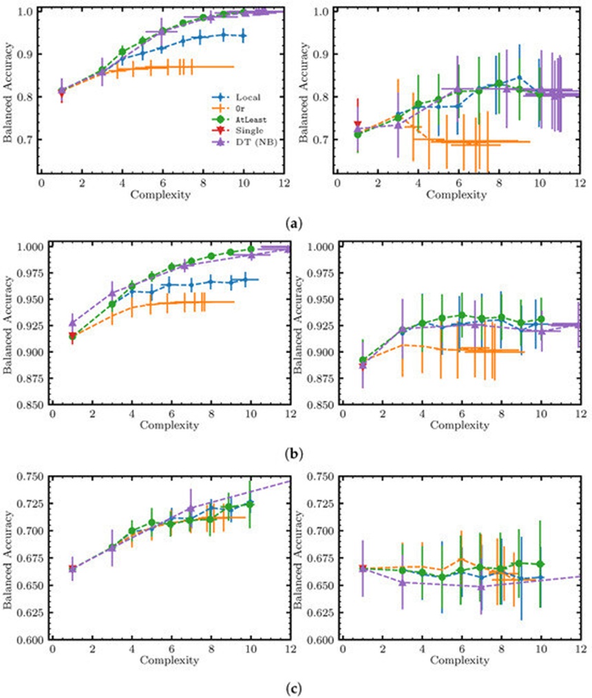
Figure 13. This graphic illustrates both the training metrics (displayed on the left) and testing metrics (displayed on the right) comparing the native local solver (“Local”) against the depth-one Or and AtLeast ILP models, the single-feature baseline (“Single”), and the unbinarized decision tree (“DT (NB)”) across the three smallest data repositories. The models underwent training and evaluation across 32 stratified, randomized shuffles using a 70/30 training/testing ratio for cross-validation on the available in-sample data (derived from an initial 80/20 stratified partition). Individual coordinates indicate the mean values for balanced accuracy and structural complexity across these 32 partitions, while the associated error bars reflect the standard deviations computed over the same splits. This data sequence extends into Figure 14. For visual simplicity, specific data lines have been left out. The sub-figures represent: (a) Parkinson’s, (b) Breast Cancer, and (c) Credit Risk.
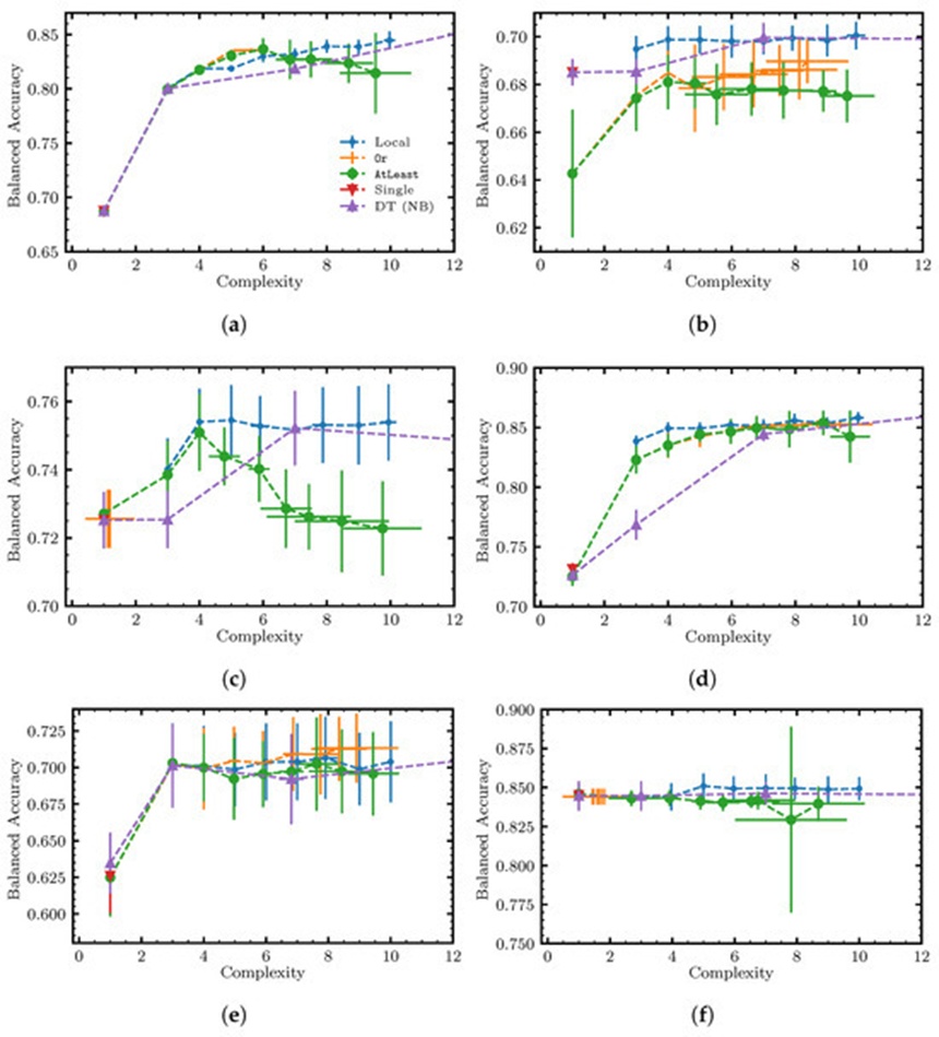
Figure 14. This visualization serves as a continuation of the data sequence introduced in Figure 13, depicting the testing performance across the six largest datasets in the study. Due to the rigorous regularization constraints inherent to these models, their training and testing performance profiles were essentially identical on these expanded datasets; because of this parity, only the testing metrics are plotted here. Certain data trajectories have been excluded to maintain visual clarity. The sub-figures represent: (a) Airline Customer Satisfaction, (b) Credit Card Default, (c) Customer Churn, (d) Direct Marketing, (e) Home Equity Default, and (f) Online Shoppers’ Intentions.
Table 4. This compilation lists illustrative logical rules produced by the native local optimization engine across each studied domain. Within this structure, the column labeled “Dataset” indicates the specific data repository, while the column labeled “Rule” reveals the highest-performing logical expression isolated during the first cross-validation partition under the constraint maxcomplexity =4. The feature terminology within these expressions is preserved directly from the source data files. Instances involving feature negations are refined during a post-processing phase by inverting the logical operator within the feature title (for instance, the expression ∼𝑎=3→𝑎≠3).
Dataset | Optimal Rule Expression |
Airline Customer Satisfaction | Conjunction And(Inflight entertainment ≠ 5, Inflight entertainment ≠ 4, Seat comfort ≠ 0) |
Breast Cancer | AtMost1(worst concave points ≤ 0.1533, worst radius ≤ 16.43, mean texture ≤ 15.3036) |
Credit Card Default | Disjunction Or(PAY_2 > 0, PAY_0 > 0, PAY_4 > 0) |
Credit Risk | Choose1(checking_status = no checking, checking_status < 200, property_magnitude = real estate) |
Customer Churn | AtMost1(tenure > 5, Contract ≠ Month-to-month, InternetService ≠ Fiber optic) |
Direct Marketing | Disjunction Or(duration > 393, nr.employed ≤ 5076.2, month = mar) |
Home Equity Default | Disjunction Or(DEBTINC > 41.6283, DELINQ ≠ 0.0, CLNO ≤ 11) |
Online Shoppers’ Intentions | AtMost1(PageValues ≤ 5.5514, PageValues ≤ 0, BounceRates > 0.025) |
Parkinson’s | AtMost1(spread1 > −6.3025, spread2 > 0.1995, Jitter:DDP > 0.0059) |
The native local rule model demonstrated competitive performance relative to the alternative classification techniques, matching the accuracy distributions of the decision tree despite the latter benefiting from a more accommodating optimization framework. While the ILP classifiers produced less complex, shallower rule structures, they achieved accuracy profiles close to the native local engine across most problem domains. However, the ILP variants required drastically longer computational runtimes, which indicates that expanding the structural depth did not consistently yield an operational advantage. Even so, certain problem domains like Direct Marketing and Customer Churn revealed a minor performance advantage for the native local optimizer, suggesting that deeper rule architectures can provide value in specific contexts. It should be kept in mind, however, that deeper rule chains generally compromise interpretability, making them less appealing for explainable AI (XAI) frameworks.
Crucially, the simple single-feature baseline matched or exceeded the performance of the more sophisticated models on the Credit Card Default, Credit Risk, and Online Shoppers’ Intentions tasks. This pattern implies that these particular problem domains demand architectures of a higher complexity than those explored in this study to unlock better performance. The top-tier accuracy scores shifted dramatically depending on the dataset under evaluation, showing that the chosen benchmarks span a wide range of operational difficulty.
On all evaluated benchmarks with the sole exception of the Parkinson’s dataset, the vast majority of the decision tree configurations generated models with such extensive structural complexity that they could not be captured within the boundaries of the plots. This pattern highlights the systematic challenge namely, that decision tree algorithms inherently scale up in structural complexity, even when the maxdepth limit is restricted to single-digit parameters.
When examining the performance variations among the different ILP operators, the evidence indicates that the parameterized configurations AtMost and AtLeast provide a distinct advantage over unparameterized alternatives, a benefit that likely stems from their greater expressive flexibility. We observe that the performance profiles of AtMost and AtLeast were nearly identical, which aligns with the functional equivalence of these two operators. Conversely, the third parameterized option, Choose, delivered weak results across multiple benchmarks. This drop in performance was likely caused by the heightened dimensionality of this particular formulation, which caused the ILP solver to hit its maximum time limits before converging on a high-quality candidate. In fact, multiple ILP iterations timed out even though the training portions of the larger datasets were downsampled to a maximum of 3,000 instances, showing that verifying absolute mathematical optimality may not scale effectively to massive data structures. Furthermore, the And operator proved more effective than the Or operator on specific benchmarks (such as the Breast Cancer data).
Sampling (RQ2)—The core intent of this analytical sequence was to determine if massive data repositories can be efficiently managed using data sampling methods—specifically, by extracting a smaller representative subset from the main data pool to execute model training (Figure 15). This line of inquiry was carried out exclusively on the three largest data repositories to provide sufficient latitude for adjusting the training sample proportions.
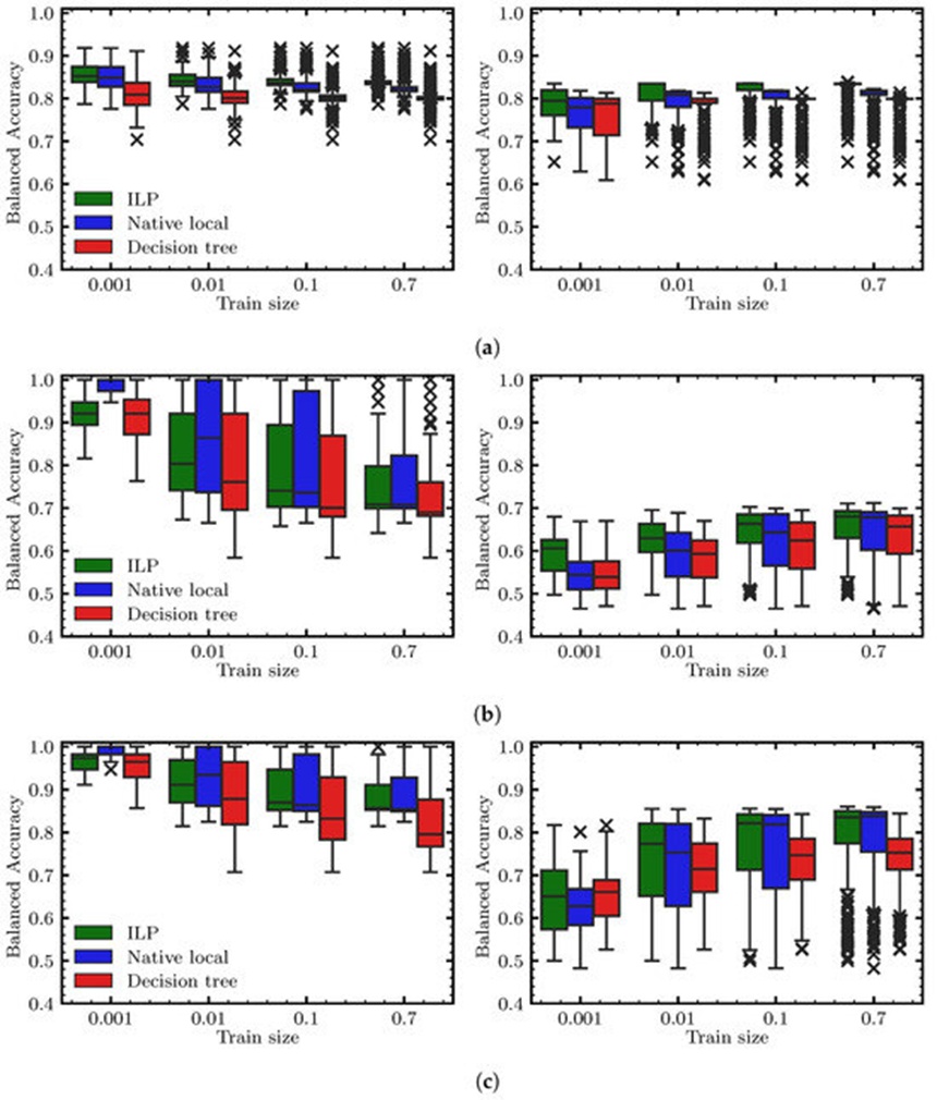
Figure 15. This visual analysis plots the training performance (shown on the left) and testing performance (shown on the right) for multiple classification models as a function of the percentage of available in-sample data allocated to the training phase. The ILP framework utilizes the Or operator under the restriction maxnumliterals =4, the native local solver operates under the constraint maxcomplexity =5, and the decision tree is restricted to maxdepth =2. For every dataset, the respective models are trained and analyzed using 64 stratified, randomized cross-validation splits of the in-sample data (originating from an 80/20 stratified split) at the designated sample sizes, with the unallocated data serves as the validation pool. The embedded box plots capture the distribution of balanced accuracy at each sequential sample size across the datasets, representing: (a) Airline Customer Satisfaction, (b) Credit Card Default, and (c) Direct Marketing.
We observed that training accuracy dropped as the training sample volume scaled upward until it hit a plateau, a trend that likely reflects the heightened difficulty of fitting larger, more diverse datasets. Simultaneously, test accuracy improved alongside the expanding training subsets, because larger sample volumes offer a superior representation of the total data space, thereby boosting generalization. The variance in performance across both the training and test sets generally contracted as the training sample size scaled up, indicating a steady convergence toward the true population score. While the training and test metrics were highly polarized at minor training sizes, they converged toward balanced values when supplied with larger training sets. These observations indicate that a few thousand instances may be fully adequate to achieve a stable performance footprint for both the ILP and native local solvers. This contrasts with contemporary deep learning methodologies that frequently demand vastly larger data volumes (such as [63]). We also emphasize that this downsampling strategy is highly attractive because of its operational simplicity and its total independence from the choice of underlying classifier.
Native non-local solver (RQ3)—The primary aim of this experiment was to isolate whether incorporating non-local optimization steps offers a tangible advantage, and to determine the precise environmental conditions where this occurs. To evaluate this, we systematically adjusted both the maxcomplexity and numiterations parameters simultaneously, as detailed in Figure 16.
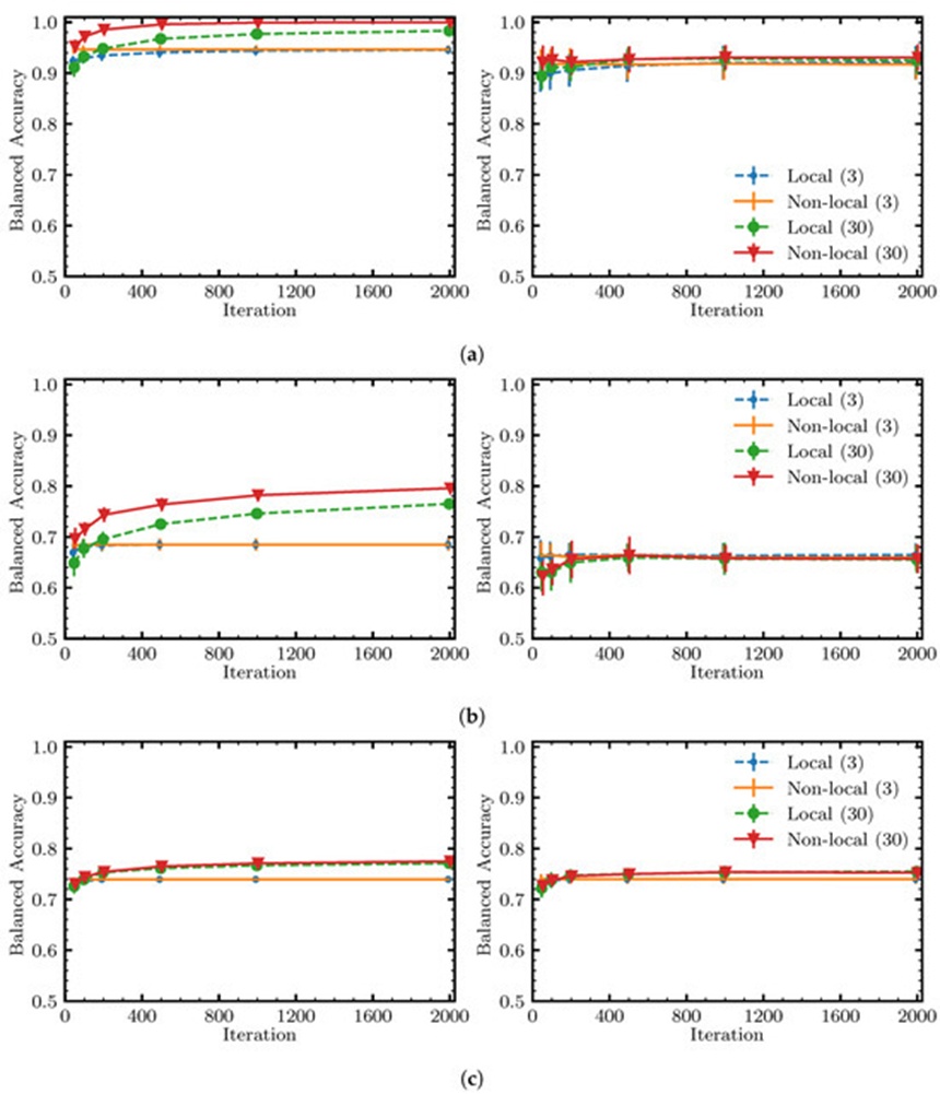
Figure 16. This pair of charts tracks the training performance (left) and testing performance (right) for the baseline native local solver alongside the enhanced native local solver utilizing non-local moves, plotted against the total iteration counts and maximum structural complexity boundaries (as defined in the chart legend). For each individual dataset, the classifiers undergo training and testing across 32 stratified, randomized shuffles of the in-sample data (drawn from an 80/20 stratified partition) at the specified training volume, while the remaining unallocated data serves as the validation set. Visual jitter has been introduced into the plotting coordinates to prevent data overlap and improve readability. The sub-figures map out: (a) Breast Cancer, (b) Credit Risk, and (c) Customer Churn.
Regarding the training metrics, the data clearly indicate that incorporating non-local steps yields a substantial enhancement (amounting to several percentage points in balanced accuracy) on two of the three evaluated datasets, alongside a nominal gain on the third. However, this phenomenon is restricted to higher complexity levels, which implies that non-local steps can be effectively leveraged to fit data using fewer optimization iterations. Assuming an optimization solver is available that can rapidly identify these non-local trajectories, its deployment could accelerate the training pipeline. Conversely, at tighter complexity thresholds, there is insufficient architectural freedom for non-local adjustments to execute, rendering them ineffective.
In terms of the test set outcomes, the associated error bars exhibit overlap, which precludes drawing definitive conclusions. Nevertheless, it is worth noting that the point estimates for the mean values show marginal improvements across the entire spectrum of model complexities for all three benchmarks.
It should also be highlighted that the highly restricted execution timeout imposed on the ILP solver when finding individual non-local steps likely constrained its capacity to locate optimal transitions. Furthermore, commercial ILP solvers generally feature a wide array of operational parameters that were left unadjusted during these trials. Directing the solver to prioritize the rapid discovery of high-quality feasible solutions would likely yield superior outcomes. We defer the exploration of this methodology to future investigations.
We have introduced the paradigm of expressive Boolean formulas, an approach prompted by the inherent structural rigidity and constrained expressivity characteristic of alternative models like decision trees and CNF rules. Building upon this framework, we introduced a novel class of interpretable machine learning classification models centered around these formulas. The optimization of these models was conducted via native local search techniques, which tolerate a highly adaptable choice of logical operators. In this implementation, native local optimization was executed utilizing a simulated annealing metaheuristic, though alternative optimization frameworks could readily be substituted.
Furthermore, the optimization process can be enhanced by executing larger, non-local transitions. In this study, such non-local moves were identified by solving an optimization subproblem formulated either as an ILP or a QUBO problem. This structural formulation introduces a viable pathway for unlocking significant computational acceleration through hardware accelerators, including prospective quantum computing platforms. While our current analysis concentrated on a depth-one configuration for non-local transitions, this could be generalized to encompass specific depth-two architectures. Additionally, the mathematical formulations developed to isolate non-local moves can function independently as self-contained classifiers, resulting in a highly shallow (depth-one) underlying Boolean rule structure.
A primary constraint of this methodology is the fundamental requirement that all incoming data features be binary. When dealing with non-binary attributes, this constraint introduces a structural dependence on the chosen binarization strategy. For specific modalities, such as image data, binarization may be conceptually ill-suited or cause a catastrophic loss of informative features. Another current limitation is that the framework is restricted to modeling a single binary output variable. In real-world applications, however, established strategies exist to extend binary classification models to handle multi-class and multi-output problems. While such extensions remain outside the immediate scope of this paper, they are integrated within the complementary Python library noted below.
To conclude, we outline several promising avenues for future research that extend beyond the boundaries of this initial study:
Datasets—The classification models introduced herein could be deployed across alternative industry domains, such as quantitative finance, clinical healthcare, and the life sciences.
Operators—The structural definition of expressive Boolean formulas—along with the execution of their corresponding classifiers—is inherently flexible by design. Consequently, specific logical operators utilized in this study could be removed, or novel operators like AllEqual or Xor could be introduced to match the unique characteristics of a given target problem.
Use cases—The core paradigm of mapping data through sequential logical operators could be adapted to alternative applications, such as digital circuit synthesis [64].
Binarization—The downstream impacts of different data binarization pipelines warrant systematic evaluation. Preliminary trials conducted with an alternative quantile-based binarization scheme (utilizing equal-count bins) yielded inferior performance, which raises the possibility that exploring alternative binarization strategies might enhance the baseline results reported here.
Implementation—Our reference implementation for the native local solver was developed in Python (the open-source version will be hosted at http://github.com/fidelity/boolxai in the near future) and did not undergo rigorous code optimization. We anticipate that the execution speed of the native local solver could be drastically improved—for instance, by rewriting the core engine in a lower-level programming language or through the strategic application of memoization techniques.
At present, quantum computing systems remain highly resource-constrained and susceptible to noise, which makes finding exact global optima computationally expensive or unfeasible even for small optimization instances. However, achieving absolute mathematical optimality is not strictly necessary for most practical explainable AI (XAI) deployment scenarios, thereby potentially relaxing the noise-tolerance thresholds required for quantum hardware. The QUBO and ILP formulations detailed in this work could, in theory, be evaluated using various quantum optimization paradigms, such as the Quantum Approximate Optimization Algorithm (QAOA) [42]. Future research may explicitly analyze the empirical performance and hardware resource constraints of quantum algorithms applied to these problems. Additionally, considerable potential exists for adapting quantum computing frameworks to other dimensions of explainable AI.
This work is a collaboration between Fidelity Center for Applied Technology, Fidelity Labs, LLC., and Amazon Quantum Solutions Lab. The authors would like to thank Cece Brooks, Michael Dascal, Cory Thigpen, Ed Cady, Kyle Booth, and Thomas Häner for fruitful discussions, and the anonymous reviewers for their feedback. H.K. would like to thank Salvatore Boccarossa for inspiration. The Fidelity publishing approval number for this paper is 1084542.1.0.
None
This research was funded by FMR LLC and Amazon Web Services, Inc.
None
Open Access The author(s) retain copyright. This article is licensed under the Creative Commons Attribution-NonCommercial-ShareAlike 4.0 International License. It may be shared and adapted for non-commercial purposes with appropriate attribution, an indication of changes, and distribution of adaptations under the same license. Third-party material may be subject to separate terms identified in its credit line. View the license at https://creativecommons.org/licenses/by-nc-sa/4.0/.
 Transparent Intelligence Publishing