Although Reinforcement Learning (RL) exhibits significant potential for refining intricate control and decision-making systems, Deep Reinforcement Learning (DRL) suffers from a distinct lack of explainability. This limitation restricts its deployment within highly regulated domains, including manufacturing, finance, and healthcare. The opacity of DRL decision-making introduces structural challenges that impede operational efficiency and resource management—an issue that intensifies alongside ongoing algorithmic advancements. While current trends favor transitioning from traditional Experience Replay configurations to A3C architectures, the latter imposes substantially greater resource demands. Furthermore, despite continuous efforts to refine selection mechanisms within Experience Replay, repository capacities generally remain elevated. In this study, we evaluate a Deep Convolutional Q-learning agent across 20 Atari environments while deliberately downsizing the Experience Replay capacity from 1×10⁶ to 5×10². Our findings indicate that lowering the capacity from 1×10⁴ to 5×10³ does not meaningfully degrade performance rewards, thereby establishing a viable strategy for resource-efficient DRL frameworks. To clarify agent choices and correlate them with inherent game mechanics, we introduce a novel methodology: visualizing the Experience Replay mechanism utilizing the Deep SHAP Explainer. This framework enhances domain comprehension and delivers transparent, interpretable accounts, though capacity constraints must be managed carefully to mitigate overfitting. Ultimately, this research validates the practicality of minimizing Experience Replay storage and supports the integration of transparent explanations via the Deep SHAP Explainer to advance resource conservation.
Over the past few years, Reinforcement Learning (RL) has developed into a robust approach for managing and optimizing intricate control workflows [1]. Nevertheless, its practical utility remains restricted in stringently regulated fields like manufacturing [2], finance [3], and healthcare [4] due to a pivotal constraint: the uninterpretable nature of Deep Reinforcement Learning (DRL). This deficit in structural transparency creates obstacles when debugging and auditing underlying decision pathways. As noted by [5, 6], such barriers frequently culminate in suboptimal model designs that exhaust system infrastructure. Furthermore, as deep learning methodologies evolve—especially regarding core frameworks like Experience Replay—the complications surrounding diagnostics, interpretability, and resource utilization are further exacerbated [7]. To mitigate these vulnerabilities, the burgeoning domain of Explainable Reinforcement Learning (XRL) seeks to deliver viable remedies. A principal asset within the XRL paradigm is SHapley Additive exPlanations (SHAP), an approach designed to quantify the specific impacts of input elements on model outputs [8].
In this study, we utilize Deep SHAP, established by [9, 10], as a complementary mechanism to map Experience Replay configurations, thereby improving the diagnostic transparency and interpretability of Deep Q-Learning (DQL). Prior literature has broadly evaluated diverse facets of DQL; for instance, [11] contrasted distinct algorithmic frameworks, Refs. [12, 13] analyzed varying selection policies, and [14] investigated the concurrent expansion of memory bounds and sampling rates starting from 1×10⁶ and 0.25, respectively. In contrast, our methodology diverges significantly. We concentrate exclusively on assessing how restricting Experience Replay capacity impacts the mean cumulative rewards generated—an optimization strategy and visualization approach that remain unexamined in prior work. Concurrently, we implement a Deep Convolutional Q-learning (DCQL) layout analogous to [14], restricting our evaluations to 20 Atari environments due to physical hardware limitations. Our objective is to identify an ideal threshold relative to the 1×10⁶ baseline of [11] or the 1×10⁴ volume suggested by [12], ensuring that the mean cumulative environment evaluation is maximized while the Experience Replay capacity M is kept at a minimum.
Within standard Reinforcement Learning (RL), the operational entity or learning architecture, designated as the Agent, operates without pre-labeled training sets to master objectives via experiential interaction. This mechanism functions through feedback in the form of a performance reward, which is provided by the surrounding environment when the Agent executes a specific action under a given scenario or state [15]. Problem resolution and operational management within this context are typically cast as a Multi-Arm Bandit (MAB), a Contextual Bandit, or a relational tuple structure known as a Markov Decision Process (MDP) [15-17]. Historically, these setups have relied on tabular matrices or grid-world configurations. The MDP framework is selected here due to its prevalence and efficacy in managing high-dimensional environments and complex, multi-stage decision sequences. Structurally, an MDP incorporates states s—represented as a feature vector or raw image sequence capturing all pertinent data at time t. It also defines a set of actions a available at time t. Additionally, it introduces a Transition Rule or state-transition probability distribution, which specifies the likelihood of shifting to a subsequent state 𝑠𝑡+1 at time t+1 based on the active state-action pair. Lastly, it defines a reward r that yields a scalar metric for taking a particular action within a given state condition. The MDP operates under the strict assumption of the Markov property, dictating that the conditional distribution of subsequent states rests entirely on the immediate state and action, independent of prior historical trajectories [18]. As detailed by [19], a variety of operational domains utilize MDP modeling, including insurance risk, retail commerce, supply inventories, and healthcare clinical admissions. The expressions below clarify the exact layout of the Transition Rule and Reward Function (Eqs. 1 and 2).
 (1)
 (2)
An Agent operating inside an MDP environment determines its actions across encountered states by adhering to a Policy 𝜋 (Eq. 3):
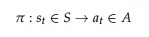 (3)
A policy serves as an operational blueprint, strategic guide, or mapping function that links state vectors to available actions. It can be constructed using stochastic actions, expert heuristics, or parameters dynamically adapted by the learning Agent. The optimal Policy 𝜋∗ (Eq. 4) selected from an available pool of policies 𝜋 is defined as the policy that yields the highest cumulative reward [16]. When analyzing or validating the outputs of a reinforcement learning pipeline, maximizing this objective function remains the primary target of the optimization process.
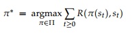 (4)
The feedback reward for each environment state within Reinforcement Learning is structurally established during the initialization of the MDP architecture (Eq. 5). The variable Gamma 𝛾 represents the temporal discount factor and is strictly bounded below 1 (with values of 0.95 or 0.99 utilized in this study). As \gamma approaches 1, the Agent increasingly prioritizes long-term returns, whereas values exceeding 1 would lead the cumulative discounted reward sequence to diverge toward infinity. Conversely, when \gamma nears 0, the agent focuses primarily on immediate localized rewards [16].
 (5)
To optimize its performance, the Agent balances exploration—navigating the environment to gather novel observations and improve future actions—with exploitation—leveraging known, high-yielding decisions. Various algorithms exist within classical Reinforcement Learning to govern these exploratory dynamics. The most straightforward exploratory techniques include A/B/n testing, Epsilon-greedy, Upper Confidence Bounds, and Thompson Sampling [15]. Other methodologies, such as Dynamic Programming (DP) via Policy Iteration and Value Iteration, compute optimal policies but require exhaustive iterations across the entire state space. While Asynchronous Dynamic Programming mitigates this issue by targeting states that have a higher probability of being visited, not all states share equal importance. Furthermore, accurately determining state transition probabilities is often difficult, making these model-reliant frameworks impractical for intricate environments. Monte Carlo approaches circumvent this limitation by deriving optimal policies directly from direct environmental interaction [15], though they generally suffer from poor sample efficiency. Conversely, model-based designs, encompassing both derivative-bearing and derivative-free techniques, achieve greater sample efficiency in specific contexts and handle model variance under sparse-data conditions by employing architectures like Bayesian Neural Networks [20] and Ensemble models [21]. While model-based paradigms excel when exploratory actions incur high real-world costs, such as in physical system control [13], they demand substantially higher computational overhead [15]. In contrast, model-free frameworks ensure high sample efficiency because they operate independently of environmental transition dynamics, learning exclusively from collected experience samples. Within this group, On-Policy and Off-Policy frameworks employ divergent exploration-exploitation mechanics during training; On-Policy techniques are better suited for scenarios with strict exploration costs or continuous action boundaries, whereas Off-Policy configurations excel at reusing historical data trajectories [15].
This study implements Q-Learning, a widely adopted model-free, off-policy algorithm derived from Temporal Difference learning. The utility of executing a particular action within a given environment state is quantified as a Q-value (𝑎,), which, prior to the adoption of deep neural networks, was tabulated within a static Q-table for every state-action combination. These Q-values are initialized to zero at t=0 and adjusted at each successive time step [16]. The Temporal Difference formula (Eq. 6) adjusts these values by computing the variance between the immediate reward combined with the discounted optimal future action, 𝑟𝑡+𝛾, and the value of the currently executed action, 𝑄(𝑎𝑡,𝑠𝑡). This Temporal Difference metric (Eq. 6) functions similarly to an internal reward signal, where higher magnitudes indicate favorable outcomes and lower values signal poor agent performance [16, 22]. It is formally expressed as follows:
 (6)
Q-Learning (Eqs. 7 and 8) extends the Temporal Difference concept (Eq. 6) by accumulating these positive and negative variance metrics for each individual state-action pair. State-action paths demonstrating elevated Temporal Difference values are reinforced, whereas paths yielding diminished values are suppressed. Consequently, the Agent learns via the Bellman Equation (Eq. 8) to converge on Q-values that yield the maximum possible Temporal Difference [23]:
 (7)
 (8)
The specific manner in which an agent interprets these Q-values depends on the exploration-exploitation mechanisms. Epsilon-Greedy and Softmax represent two prominent frameworks with distinct operational nuances [24]. The Epsilon-Greedy technique is a straightforward exploratory framework that primarily selects actions with the highest value estimates while occasionally picking arbitrary alternatives based on a minor epsilon probability factor. Softmax exploration operates probabilistically, allocating action probabilities proportional to their estimated Q-values. While Epsilon-Greedy functions in a binary manner, the Softmax mechanism (Eq. 7) deployed in this study provides a smoother exploratory trajectory by distributing selection probabilities across all viable actions governed by a Temperature parameter T, smoothly balancing exploration and exploitation [16].
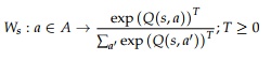 (9)
The subsequent Section delineates Deep Q-Learning and its corresponding implementations, wherein the classical matrix-based Q-table is substituted with a neural network value function approximator.
Deep Q-learning
Deep Q-Learning (DQL), which incorporates the foundational Bellman Equation (Eq. 8) [23], enables the optimization of control architectures inside highly complex environments [17], such as mastering video games directly from raw pixel streams [11]. Through iterative trial-and-error interactions, the DQL agent evaluates the utility of taking actions within an MDP-structured environment to establish an optimal behavioral policy that maximizes cumulative reward metrics. The inputs supplied to the neural network consist of state representations, while the output layers yield estimated Q-values. Applying either Epsilon-Greedy or Softmax functions to this output layer translates these continuous Q-values into distinct behavioral actions. The network is optimized using backpropagation guided by the Bellman Equation (Eq. 8). Here, the target ground-truth value y represents the highest anticipated future q-value, whereas the predicted value \hat{y} is generated by the neural network based on the active state inputs. For vector data arrays native to tabular or grid-world RL setups, basic feedforward neural architectures suffice; however, image-based domains like those evaluated in this study demand convolutional neural networks. The one-dimensional flattened layer containing features extracted from the state image is fed into a neural network that calculates Q-values, which are subsequently processed by Epsilon-Greedy or Softmax selection routines to determine the agent's action.
To properly capture directional movement and velocity in visual environments, a single static frame is insufficient; hence, a chronological sequence of images must be evaluated. When training an agent in a simulation, a sequence of n-steps up to time t is utilized (with this research specifying n=10). Under these conditions, Eligibility Traces can be implemented during training. This methodology assigns credit to historical actions across a sequence of states and actions to update the underlying weights of the neural network model [25]. This approach mitigates the challenges associated with delayed rewards and facilitates successful optimization in environments characterized by significant temporal gaps between an action and its eventual consequences, which is essential for mastering intricate, pixel-driven video games. Throughout the optimization pipeline, the Eligibility Trace is modified at each n-step interval by applying a decay factor and adding the weight gradients relative to the loss function. When a parameter update occurs, the Eligibility Trace dictates the proportion of credit assigned to each individual weight based on its historical influence on the current state outcome. By aggregating these Eligibility Traces over time, the algorithm successfully attributes credit to foundational actions that yield distant future rewards, even when those rewards are highly delayed.
Deep Reinforcement Learning (DRL) inherently requires substantially larger volumes of training data than standard deep learning applications [15]. Intricate models routinely require months of training spanning millions of operational iterations. Because collecting such massive datasets empirically is impractical, DRL remains heavily dependent on simulated environments. This dependency introduces several complications into DRL workflows. Many industrial sectors lack accurate simulated models of their proprietary operations. When available simulations are overly simplistic, the DRL model often overfits to the idealized virtual parameters and fails when deployed in real-world settings. Addressing this issue requires calibrating the simulation to mirror real-world parameters closely, as machine learning models require identical training and testing distributions; however, tuning a simulation is both costly and labor-intensive, a challenge widely known as the "Sim2real" gap. Enhancing the fidelity of a simulation increases computational overhead, which hinders rapid experimentation and deployment. Furthermore, many simulation platforms lack generalization; various commercial software applications are difficult to interface with DRL architectures or lack the flexibility required to support these models. As noted in [15], simulations must be high-speed, mathematically precise, and capable of scaling across numerous concurrent sessions. Virtual environments are essential for safely replicating real-world complexities and generating high-fidelity training data [26]. This study utilizes video games for model optimization due to their explicit rule structures and sufficient complexity to mirror real-world challenges. DQL is widely applied across computer gaming, autonomous driving, recommendation engines, robotics, power grid management, financial fraud detection, dynamic pricing models, and clinical healthcare [1], where performance benchmarking involves comparing an Agent's output against hardcoded heuristics, human experts, or stochastic baselines. This paper benchmarks the Agent against its own historical profiles operating under varied Experience Replay buffer dimensions.
Approximating continuous Q-values with neural architectures in expansive, high-dimensional states—such as autonomous driving, medical systems, or video games—can destabilize the optimization process. To counter this, [11, 27] integrated an Experience Replay mechanism [28] to store and randomly sample environmental data transitions for subsequent reuse by the value function approximator. Nonetheless, this approach introduces vulnerabilities, including highly correlated data samples, limited buffer capacities that cause the agent to overwrite older information, outdated transitions resulting from non-stationary environments, and overfitting due to the memorization of specific samples. Prioritized Experience Replay (PER) [29], Attention-Based Experience Replay [30], Combined Experience Replay (CER) [12], and Explanation-Aware Experience Replay [31], alongside various alternative selection methodologies [12-14, 32], have been proposed to mitigate these limitations.
A comprehensive understanding of Experience Replay dynamics is essential for operational efficiency. The framework in [11] required 1 million frames of experience to surpass human baselines across 49 Atari environments, while DeepMind’s advanced Agent57 architecture [33], which outperformed human champions on Atari, required 80 billion operational experience frames to achieve peak performance. Consequently, Experience Replay is frequently viewed as structurally flawed, with some researchers seeking alternatives because the likelihood of any newly generated transition being replayed decreases monotonically as buffer capacity expands [12]. The Asynchronous Actor-Critic (A3C) framework by [27] represents a prominent alternative. It coordinates multiple agents in parallel to navigate the environment and update a centralized network, which demands greater hardware resources but accelerates convergence rates.
A broader trend in deep learning indicates that performance gains are frequently achieved at the expense of massive hardware scaling. For example, the image classification network AlexNet, which trained for 5 to 6 days across two GPUs in 2012, was surpassed by NASNet-A in 2018; the latter halved the error rate but required a 1000-fold increase in computational processing [7]. Experience Replay, despite its slower throughput, remains structurally more memory-efficient, requiring only stored data transitions rather than multiple operational duplicates of the network architecture. It was emphasized by [12] that the Experience Replay capacity M remains a largely overlooked hyperparameter that can degrade agent performance if excessively large; the authors noted that most implementations default to the 1M transition capacity established by [27]. Although [12] did not evaluate how Experience Replay interacts with a Deep Convolutional Network, they introduced CER as a selection framework to counteract the negative effects of large buffer sizes, offering greater efficiency than PER. Additionally, [13] evaluated how the utility of distinct experiences is affected by the underlying control problem, offering framework guidelines to leverage prior domain knowledge when choosing an experience selection strategy. As a general rule of thumb, [13] recommended maintaining a high Experience Replay capacity that retains 90% of the total environmental transition steps. Because [11] utilized 50 million frames of environmental transitions, this 90% guideline would dictate a buffer size of 45 million transitions rather than the standard 1 million. Conversely, [14] demonstrated within the Atari Learning Environment that expanding the Experience Replay capacity from 1 million to 10 million transitions while reducing the operational age of the oldest policy improved overall agent performance. However, scaling down the Experience Replay capacity threatens data integrity, particularly in complex, rule-dense environments, and as demonstrated by [13, 31], any expansion of the Experience Replay buffer places an additional burden on computational infrastructure [5, 6].
Explainable Artificial Intelligence (XAI) concentrates on demystifying the internal mechanics of autonomous systems, translating complex computational pathways into formats accessible to human operators. For frameworks like Deep Q-Learning to achieve broader industrial integration, it is necessary to enhance diagnostic methodologies and clarify how their underlying choices are made. Implementing XAI is critical for establishing operational trust, ensuring corporate accountability, fulfilling regulatory mandates, and maintaining ethical standards [34]. A diverse array of methodologies has been formulated to achieve such transparency [34-36]. A frequent practice relies on post-hoc analytical frameworks, which dissect and clarify decisions after a network has generated its predictions. Saliency mapping, feature importance visualizations, and SHAP (Shapley Additive exPlanations) represent primary examples of this technique [34]. Additionally, researchers are developing hybrid architectures that pair high-capacity models with specialized interpretability modules. Tools such as TreeExplainer—a tailored variant of SHAP optimized for tree-based machine learning—and combinations of SHAP with Lorenz Zonoids decomposition serve to isolate critical variables by constructing receiver operating characteristic (ROC) curves.
This research integrates Deep Explainer (Deep SHAP), a hybrid paradigm that merges the DeepLIFT (Deep Learning Important FeaTures) algorithm [9] with SHapley Additive exPlanations (SHAP) [10]. DeepLIFT unpacks the final prediction of a neural network for a specific input by backpropagating internal neural contributions back to each initial input dimension, while SHAP reconstructs individual outcomes by measuring the marginal impact of every feature for a specific instance. To illustrate, a salary forecasting model might establish a baseline estimate of €50 per hour given three input variables: age, gender, and experience. If the final model projection drops to €40 per hour, individual inputs are systematically removed to isolate their marginal variance; this process might reveal that the age variable introduces a negative impact of −€10 per hour relative to the baseline. The Deep SHAP framework approximates these values by establishing explicit structural alignments with DeepLIFT and optimizing across a background distribution of reference samples rather than anchoring to a single static baseline. In a standard Deep SHAP visualization, the primary input frame is presented in a muted, transparent grayscale, overlaid with distinct color bands indicating localized feature impacts. Red pixels highlight regions that drive a positive increase in the network's output value, whereas blue pixels denote regions that lower the target estimation. The total summation of these SHAP metrics matches the variance between the baseline model output (calculated as an average across the background reference image set) and the localized prediction. Within a Deep Convolutional Q-Learning architecture, this maps to an active game frame paired with projected Q-values for each available action, extending a set number of n-steps into the future. For example, a resulting SHAP heatmap can visually isolate why a particular maneuver achieves an elevated q-value; in SpaceInvaders, this might occur because the agent anticipates the arrival of a mothership, causing it to prioritize firing into an unpopulated coordinate sector to intercept the vehicle and secure a 300-point reward.
The absolute minimum capacity threshold for an Experience Replay buffer in DQL remains an open question. However, using Deep SHAP diagnostics alongside a controlled downscaling of this memory repository can illuminate core algorithmic behavior, training trajectories, and hidden performance traits, bringing anomalies or novel behavioral motifs to light for deeper study [10, 34-36]. While several specialized explainability frameworks have been engineered for DQL [37-40] to interpret in-game scenarios or the agent's actions within them, these tools do not address the archived experience transitions that the network extracts as training inputs to calculate Q-values. Within Explainable Reinforcement Learning (XRL) [5, 8, 41], SHAP [10] remains a primary choice for black-box decomposition [39, 40, 42]. Although RL-SHAP diagrams have been deployed to clarify grid-world environment features and their downstream effects on action selection, they have not yet been implemented for pixel-driven environments or applied directly to the historical samples archived inside an Experience Replay cache. Similarly, while an Experience Replay repository can be partitioned into distinct sub-clusters and assigned semantic labels based on local rule density to filter environment inputs [31], this acts purely as an experience selection strategy rather than a post-hoc diagnostic tool for debugging an active DCQL model. This paper introduces the use of Deep SHAP Explanations to generate visual mappings of Experience Replay states, revealing hidden patterns and behavioral tendencies to assist in auditing the DQL pipeline as its buffer capacity is reduced. The following section details a primary empirical study focused on establishing a minimum Experience Replay boundary in Deep Q-Learning and using Deep SHAP to monitor these internal repositories throughout the optimization process.
To evaluate how varying Experience Replay capacity bounds influence mean cumulative rewards, we structured a primary empirical experiment. This section covers the components of data understanding, preparation, modeling, and evaluation that define this research layout.
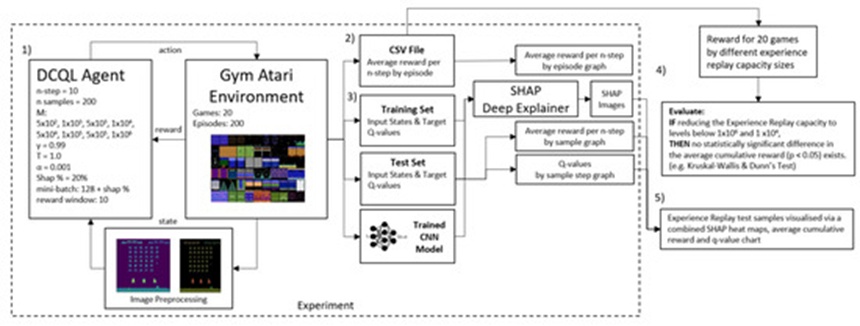
Figure 1. The comprehensive design of the experimental workflow involves several sequential stages. First, the DCQL agent is executed inside the target Atari simulation to compile an initial evaluation dataset. This collected data is then written to a static CSV file to facilitate subsequent analytical reviews. Next, novel, unexamined data points are pulled from the Experience Replay buffer to train the convolutional neural network; these data points are split into distinct training and testing partitions, which are also used to initialize the Deep SHAP Explainer. Following this setup, performance metrics are gathered across 20 distinct games to isolate the specific Experience Replay buffer volume that yields the highest mean cumulative score. Finally, visual diagrams are extracted from the SHAP Deep Explainer, allowing for a direct comparison between the spatial heatmaps, estimated Q-values, and the raw rewards captured during the agent's optimization timeline.
To gather reward outputs across distinct Experience Replay capacities, an agent driven by a convolutional neural network processes incoming state vectors and derives corresponding Q-values for each potential option. The agent then executes selected actions to manipulate the simulation state and refresh the incoming data. The operational testbed is the Atari Arcade Learning Environment, paired with the OpenAI Gym interface [26, 43]. The Atari titles run via the Stella emulation core, providing a secure sandbox that mimics complex, real-world control challenges to generate useful training logs. This research spans 20 specific titles: AirRaid, Asterix, Asteroids, Bowling, Breakout, DemonAttack, Freeway, Gravitar, Jamesbond, Montezuma Revenge, MsPacman, Pong, PrivateEye, Qbert, Seaquest, SpaceInvaders, Venture, WizardOfWor, Yar’s Revenge, and Zaxxon. The agent's operational competence is measured by benchmarking its accumulated score against its own prior historical policies, a handcrafted human expert baseline, or a purely stochastic policy. Within OpenAI Gym, each game environment introduces an independent set of states, action spaces, and reward distributions. State information is supplied directly as raw pixel streams. Actions are represented as discrete integers, covering directional movements, static positioning, or firing mechanisms. Every environment maintains a unique objective and scoring architecture. In SpaceInvaders, for example, rewards scale with each standard opponent eliminated, featuring a premium payout for downing the mothership; Breakout utilizes a paddle and ball system to dismantle a wall of bricks; and Montezuma Revenge demands complex spatial planning, requiring the agent to traverse a castle layout, collect keys to unlock barriers, gather treasure items, and avoid hostile units.
At each discrete interval t, the simulation environment delivers updated state data and an associated scalar reward to the agent. During the initial phases of execution, this reward signal can drop below zero to incentivize active engagement; without this mechanism, the agent might inadvertently discover that remaining entirely motionless is the most effective way to avoid negative feedback. As the agent selects actions, it encounters shifting positive and negative reward signals, and the emulation platform updates the observation array immediately following every choice. OpenAI Gym provides the interface needed to capture these data streams at each chronological step.
Visual States: Supplying raw images directly to the agent without preliminary preprocessing leads to prolonged training times without yielding parallel performance benefits. Consequently, each input frame is downscaled from its default resolution, following the foundational methodology outlined by [11] (for example, standard Atari SpaceInvaders provides 210 px, 160 px, 3 color channels) to a compressed grayscale matrix (specifically 80 px, 80 px, 1 color channel). To preserve velocity data and directional indicators, frames are accumulated and batched before being fed into the deep convolutional Q-learning engine. The temporal batch size is locked at 10, meaning the agent completes 10 consecutive environmental updates before those 10 images are clustered and logged in a history buffer for downstream use. By comparison, [11] enforced an n-step value of 4, [12] used an n-step value of 1, and [14] evaluated ranges spanning from n-step = 2 to n-step = 7.
Discrete Actions: If the configuration space restricts movement to left, right, up, and down, the environment registers the agent's discrete action capacity as 4. Every unique simulation contains its own hardcoded action boundaries, with certain Atari environments supporting up to 14 discrete actions.
Data Sampling: A mini-batch consisting of 154 random data instances is extracted from the agent's Experience Replay buffer. From this subset, 128 instances serve as direct training inputs for the agent, while the remaining 20% is isolated as an independent test set used downstream to calibrate the SHAP Deep Explainer.
The data preprocessing workflow detailed in this section remains uniform across all evaluations. This structured data is subsequently used to train a convolutional neural network designed to estimate Q-values, as outlined in the following section.
The DCQL framework detailed in this section replicates the original Deep Q-Learning model proposed by [11]. It is structured to process intricate state patterns supplied in raw pixel format. The conceptual design of the DCQL Agent's pipeline is illustrated in Figure 2, utilizing 3 distinct convolutional hidden layers.
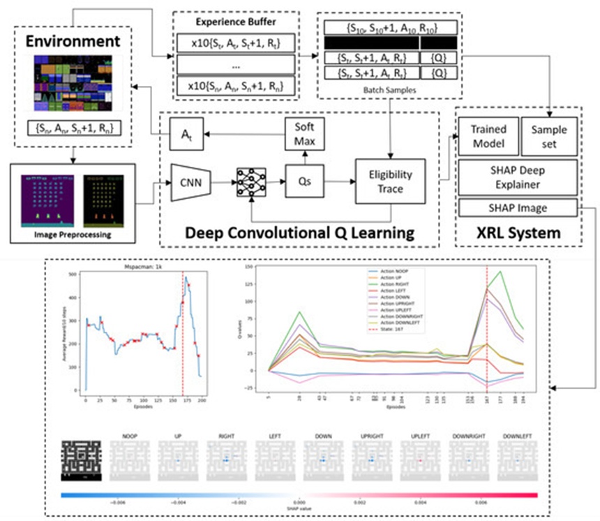
Figure 2. DCQL Architecture: (1) The active Agent executes 200 distinct actions per training episode. (2) The simulation returns a scalar reward value alongside the subsequent state vector. A total of 10 preprocessed frame observations are logged inside a temporal n-step history buffer. (3) Transitions held within the memory repository are randomly sampled 154 times, splitting into a 128-sample training subset and a 26-sample validation subset. (4) A convolutional neural network models action-value functions, generating the subsequent optimal action using a Softmax selection function. (5) This execution routine is repeated over a span of 200 episodes, and 20 validation transitions are pulled from the memory repository. (6) The underlying CNN parameter configuration is preserved. (7) A Deep Explainer module constructs interpretable SHAP feature metrics.
The initial convolutional layer processes a solitary 80 × 80 pixel frame input feature, projecting 32 independent activation feature maps scaled to 5 × 5 dimensions.
The secondary layer ingests these 32 feature maps and outputs a condensed set of activation representations mapped to 3 × 3 pixel dimensions.
The terminal convolutional hidden layer acts on these intermediate feature maps to output 64 final feature matrices scaled to 2 × 2 dimensions.
The computational tensors extracted from these convolutional processes are routed directly into a fully connected feedforward layer, where the initial array of input nodes is calculated dynamically. This target quantity is established by propagating a synthetic, completely blank black-and-white matrix (80 px × 80 px) through the 3 convolutional stages using a maximum pooling mechanism governed by a stride parameter of 2, followed by flattening the resulting tensors into a single-dimensional vector. This operation outputs the exact number of input connections needed for the linear layer.
As previously established, a standard downsampling pooling layer is omitted from the convolutional blocks to preserve the exact spatial coordinates of visual elements within the frame. A hidden layer containing 40 individual neurons links this representation to a second fully connected linear layer. The output nodes represent estimated Q-values matched to the number of discrete actions available to the Agent. These calculated Q-values are then evaluated by a Softmax Policy to balance exploratory and exploitative choices during action selection. The DCQL Agent optimizes its parameters via an Eligibility Trace routine. This setup is mathematically analogous to the Asynchronous n-step Q-learning framework detailed by [27], with the modifications that a Softmax policy replaces the standard Epsilon-Greedy approach, and an Experience Replay buffer is implemented instead of the parallel A3C network layout.
Converging on optimal behavior within Atari environments frequently requires extensive operational iterations. For example, when the baseline DCQL Agent in [11] was trained on Atari SpaceInvaders to outperform human scoring benchmarks, the optimization process required between 10 × 106 and 40 × 106 operational steps. To accommodate localized hardware configurations and strict temporal limitations, the execution boundary for each game in this study was set to 200 episodes, matching the experimental duration used in [14], which limited training time to approximately one hour per game simulation. An individual episode encompasses numerous environment updates, running continuously until a predefined terminal state occurs (e.g., the temporal limit expires or the Agent triggers a loss condition). Within the Atari SpaceInvaders environment, a terminal threshold is reached when the player's entity is eliminated by hostile units.
An informal diagnostic evaluation of each game indicated an average of approximately 2000 environment transitions per episode. From each episode, 200 baseline state observations are extracted, with each independent sample spanning 10 distinct chronological intervals (n = 10). This configuration yields an aggregate of 4 × 10^5 steps during which rewards are generated in response to executed actions. Upon reaching a terminal state, the total accumulated reward is logged. A moving average is then computed using a temporal window size of 10 steps, following the evaluation approach in [14]. At the initialization of each game environment, the Experience Replay storage bound is set to an initial baseline of 1 × 10^6 and systematically downscaled to setpoints of 5 × 10⁵, 1 × 10⁵, 5 × 10⁴, 1 × 10⁴, 5 × 10³, 1 × 10², and 5 × 10² stored transitions, respectively.
Once performance rewards are compiled for each localized Experience Replay capacity across the 20 Atari titles, the data is exported to a static CSV file. Following the completion of all game environments, these independent CSV arrays are consolidated. An Analysis of Variance (ANOVA) model or its non-parametric counterpart, the Kruskal-Wallis test, is executed alongside an appropriate post-hoc pairwise assessment (either Tukey's honestly significant difference or Dunn's test) on the resulting reward distributions. The selection of the standard parametric ANOVA over the non-parametric Kruskal-Wallis framework is governed by a preceding Shapiro-Wilk test to confirm whether the underlying performance reward metrics adhere to a normal distribution.
This research examines how systematically restricting the Experience Replay buffer volume beneath both the traditional baseline of 1 × 10⁶ used by [11] and the common empirical threshold of 1 × 10⁴ (analyzed in [12-14]) influences mean accumulated rewards within a Deep Q-Learning framework across 20 Atari titles. This paper hypothesizes that minimizing the Experience Replay capacity below these established benchmarks will not yield a statistically significant variance in mean cumulative performance rewards at an alpha level of p < 0.05 when directly compared to the baseline tracking volumes of 1 × 10⁶ and 1 × 10⁴. Confirming this hypothesis would indicate that the Experience Replay capacity hyperparameter M can be safely reduced without causing a drop in agent performance. Formally, this hypothesis is specified as follows:
To empirically evaluate this research hypothesis, the following statistical validation methods are used:
One-Way Analysis of Variance (ANOVA): This parametric procedure is implemented to determine the presence of statistically significant variances among the mean values of independent, unlinked reward groupings. These groupings are defined by their unique Experience Replay capacity configurations, initialized at 1×10⁶ and systematically restricted to step-downs of 5×10⁵, 1×10⁵, 5×10⁴, 1×10⁴, 5×10³, 1×10², and 5×10² transitions, respectively.
Shapiro-Wilk Test: This normality check is used to validate the mathematical prerequisites of the downstream analysis. It determines whether the accumulated performance reward data conforms to a standard normal distribution, which is a required condition for running an ANOVA and subsequent Tukey comparisons rather than falling back on a Kruskal-Wallis pipeline paired with Dunn's post-hoc tests [44].
Kruskal-Wallis Test: This non-parametric statistical approach operates directly on data ranks rather than raw values. By pooling data across all test groups and converting scores into ordinal ranks, it generates a test statistic that evaluates variances among the ranked group medians, mirroring the comparative function of an ANOVA. This resulting test statistic closely approximates a chi-squared distribution with (k - 1) degrees of freedom, where k represents the total number of independent capacity groups under review. The null hypothesis states that median performance values remain identical across all Experience Replay capacities, while the alternative hypothesis states that at least one capacity configuration produces a distinct median distribution [45].
Tukey Test: This post-hoc pairwise comparison framework is deployed following a significant ANOVA result. While the omnibus ANOVA indicates whether an overall variance exists among group means, Tukey's test isolates which specific pairs of Experience Replay capacities display statistically significant performance differences.
Dunn’s Test: This post-hoc validation tool performs a role similar to Tukey's test but is designed for non-parametric workflows following a Kruskal-Wallis evaluation. It isolates and highlights which specific Experience Replay capacity boundaries exhibit significant variations in their underlying score distributions.
Figure 3 contrasts the performance distributions of the first experimental cluster (5×10⁵, 1×10⁵, 5×10⁴) with the baseline standard of 1×10⁶, alongside the second cluster (5×10³, 1×10², 5×10²) evaluated against the secondary benchmark of 1×10⁴. The outlying data points shown in this distribution represent authentic, unedited performance tracks across the 20 Atari test environments, capturing specialized scenarios where specific titles generated substantially higher scores than the global average. An evaluation of the median lines and interquartile distributions indicates an apparent divergence in central tendencies between the 1×10⁶ baseline and the remaining memory conditions. Interestingly, however, the 103 and 1×10⁴ buffer settings exhibit nearly identical mean values, prompting deeper statistical verification. The subsequent text details the outcomes of the Shapiro-Wilk normality check, the Kruskal-Wallis analysis, and Dunn’s post-hoc evaluation. The Shapiro-Wilk test (p<0.001) indicates that the standard parametric normality prerequisites for an ANOVA are violated; consequently, a non-parametric Kruskal-Wallis Test (p<0.001) was implemented, demonstrating a significant statistical variance across the capacity groups. Table 1 presents the matrix derived from Dunn’s Post Hoc Test, where the rows denote the source evaluation groups and the columns represent the target comparison groups. Individual cell entries provide the exact p-values for the localized pairwise comparisons between the corresponding source and target categories. Diagonal intersections are uniformly populated with values of one since the source and target configurations are identical.
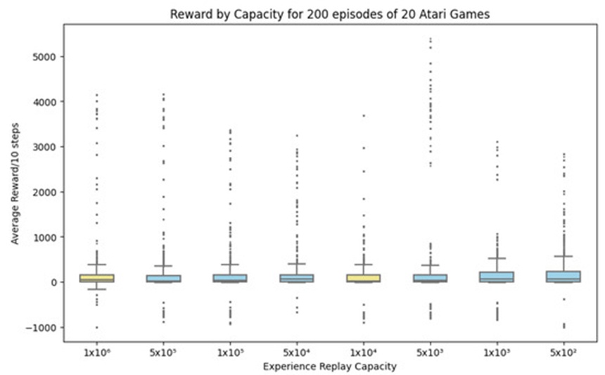
Figure 3. Score Profiles across Memory Conditions: This boxplot maps the variations in accumulated agent rewards when evaluated under the primary baseline (1×10⁶) and secondary control threshold (1×10⁴), directly contrasting them against the primary downscaled configurations (5×10⁵, 1×10⁵, 5×10⁴) and the highly restricted storage allocations (5×10³, 1×10², and 5×10²).
Table 1. Dunn’s Post Hoc Test.
| 1×10⁶ | 5×10⁵ | 1×10⁵ | 5 x 10⁴ | 1x10⁴ | 5 x 10³ | 1 x 10³ | 5 x 10² |
1×10⁶ | 1.000 | 0.001 | 0.111 | 0.017 | 00003 | 0.003 | <0.001 | <0.001 |
5×10⁵ | 0.001 | 1.000 | 0.090 | 0.715 | .722 | <0.001 | <0.001 | <0.001 |
1×10⁵ | 0.111 | 0.090 | 1.000 | 40.001 | 0.181 | 0.184 | <0.001 | <0.001 |
5 x 10⁴ | 0.017 | 0.715 | <0.001 | 1.000 | <0.001 | <0.001 | 0.009 | 0.001 |
1x10⁴ | 0.003 | 0.722 | 0.181 | 40.001 | 1.000 | 0.993 | <0.001 | <0.001 |
5 x 10³ | 0.003 | <0.001 | 0.184 | 40.001 | 0.993 | 1.000 | <0.001 | <0.001 |
1 x 10³ | 0.001 | <0.001 | <0.001 | 0.009 | <0.001 | <0.001 | 1.000 | 0.480 |
5 x 10² | 0.001 | <0.001 | <0.001 | 0.001 | <0.001 | <0.001 | 0.480 | 1.000 |
Note: Symmetric cells omitted for clarity; cell intersections dictate the pairwise p-value metrics.
Based on the localized Dunn’s Post Hoc Test matrix detailed in Table 1, the mathematical intersection between the 1×10⁴ control and the restricted 5×10³ capacity yields an approximate value of p=0.993. Intersections linking identical rows and columns return values of 1.000, confirming the absence of internal variance as expected. Consequently, the derived p-value for the comparative analysis between the buffer boundaries of 10,000 and 5000 transitions approaches unity, proving that there is no statistically significant variance in cumulative score averages across the 20 Atari test environments for these two groups.
To execute this evaluation, the DCQL Agent was deployed across 20 distinct Atari environments. The Kruskal-Wallis framework and Dunn's pairwise testing were chosen because the collected reward distributions violated the Shapiro-Wilk normality criteria required for a standard ANOVA. The baseline null hypothesis of the Kruskal-Wallis evaluation was successfully rejected, demonstrating that variance (p < 0.05) is introduced into reward values when the Experience Replay buffer is downscaled. However, the subsequent post-hoc Dunn’s analysis isolated 5×10³ transitions as the minimum sustainable Experience Replay threshold across the 20 Atari games (Table 1). As demonstrated by the distribution trends in Figure 4, the core DCQL design lacked the architectural capacity to achieve high scores, and specific game titles proved too structurally complex to yield distinct performance records (notably Montezuma’s Revenge and Venture). Memory management using uniform random sampling represents a suboptimal storage strategy [12-14, 29-32], and restricting Experience Replay capacity introduces a structural hazard where high-density behavioral rules might be overwritten; nonetheless, buffer capacity can be systematically reduced from 1×10⁴ to 5×10³ without causing a severe decline in performance rewards. This reduction enhances operational efficiency by minimizing the agent's impact on system resources.
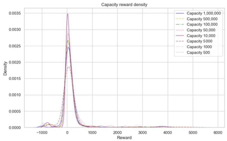
Figure 4. Score Probability Distributions: This probability density chart maps performance metrics across every individual buffer size, demonstrating that the curve peaks heavily near zero. This visualization confirms that the underlying model struggles to achieve high scores across the selected games due to uniform random data selection limits, an extensive temporal stack (n\text{-step} = 10), or an overly exploratory action policy (Softmax T = 1.0). Crucially, the graph highlights that the restricted 5×10³ configuration exhibits a minor performance advantage over the traditional 1×10⁴ threshold.
The remainder of this section analyzes the data gathered by visualizing the Experience Replay system using the Deep SHAP Explainer framework. Maps containing localized SHAP weights were examined to determine whether the Agent's decision-making process at the minimal capacity boundary functions correctly—meaning the model has extracted the primary operational mechanics of the simulation—and to isolate which performance outliers might be distorting the global metrics. These visual captures are not presented as direct proof for the underlying hypothesis, but rather as graphic representations of the behavioral trends and tracking outcomes observed throughout the training pipeline. The 20 evaluation titles managed by the DCQL architecture consisted of AirRaid, Asterix, Asteroids, Bowling, Breakout, DemonAttack, Freeway, Gravitar, Jamesbond, Montezuma Revenge, MsPacman, Pong, PrivateEye, Qbert, Seaquest, SpaceInvaders, Venture, WizardOfWor, Yar’s Revenge, and Zaxxon, with specific analytical focus directed toward MsPacman.
In the localized MsPacman environment profiles shown in Figure 5, buffer boundaries fixed at 1 million or 100,000 transitions yield score records that outperform alternative settings, with the notable exception of the 1000 capacity threshold. At this specific 1000-transition step-down, the DCQN Agent appears to prioritize immediate rules using recently acquired operational experiences, rather than storing and iterating over historical transition data. Leveraging the SHAP architecture allows us to review sample frames extracted from this 1000-capacity buffer at specific milestones along the training timeline to evaluate the underlying factors driving the DCQN's choices. Two notable milestones chosen for detailed analysis are episode 167 (Figure 6) and episode 177 (Figure 7).
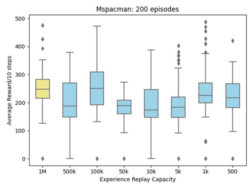
Figure 5. Performance Dispersion in MsPacman: This box-and-whisker plot illustrates the range of rewards secured across the MsPacman environment during 200 consecutive training episodes per trial, tracking the localized performance effects of systematically reducing the underlying Experience Replay capacity.
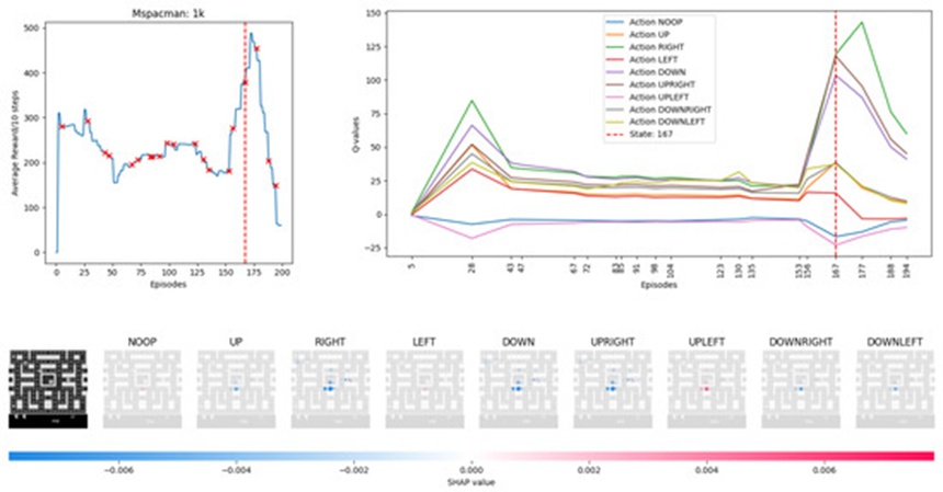
Figure 6. MsPacman Diagnostic Frame (Episode 167): This multi-panel plot captures the agent's state immediately prior to achieving a significant reward influx. The line graph tracking cumulative score uses red markers to indicate where uniform memory snapshots were taken to train the feature importance framework, while the vertical dashed reference line identifies the specific runtime instance decoded below by the Deep SHAP visual grids.
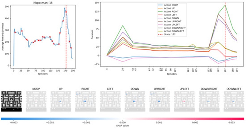
Figure 7. MsPacman Diagnostic Frame (Episode 177): This multi-panel diagnostic layout tracks the agent's performance profile across 200 episodes for each independent memory boundary condition. Red markers on the primary score timeline pinpoint the precise instances where random experiences were archived for explainability profiling, and the vertical dashed indicator denotes the active timeframe rendered via the localized Deep SHAP grids. This visualization illustrates that while large storage footprints (1 million and 100,000 transitions) generally yield higher scores, the heavily downscaled 1000-transition configuration matches this performance by prioritizing recent, immediate transitions rather than iterating over stale historical data.
Evaluating the tracking path in Figure 6 indicates that the agent's prior actions were successful in increasing the cumulative reward. Red markers on the performance axis denote the specific instances where stochastic frames were extracted from the Experience Replay repository to initialize the Deep SHAP Explainer. The vertical dashed marker highlights that episode 167 is the active frame under review. The adjacent line graph tracks the real-time adjustments made to estimated Q-values as the DCQL model attempts to extract meaningful updates from the transitions gathered within its environment. The lower section of Figure 6 displays the calculated SHAP values overlaid directly onto the game frames relative to a baseline reference state. Reviewing this structural layout shows that the DCQN agent initiated its trajectory in the center before navigating upward and toward the right quadrant. Each of the 9 actions available within this game environment is displayed individually. Blue pixel overlays highlight regions that negatively influence the expected Q-value calculation, whereas red pixel groupings denote fields that exert a positive influence. The intensity of these color fields corresponds to the magnitude of their influence on the network, the direct results of which are reflected in the shifting lines on the Q-value tracking graph. These output Q-values are balanced by the Softmax selection rule; consequently, a high action-value estimate may not automatically trigger execution depending on the active temperature parameter T, but an elevated Q-value ensures a higher mathematical probability that the corresponding action will be selected.
Taking the UPLEFT maneuver shown in the 7th image from the left of the Deep SHAP matrix in Figure 6 as a case study, we can observe that this action was previously penalized by the network but has now been assigned high execution priority. The Agent is replaying its recorded trajectory of moving from the lower-left sector toward the center-right region; it evaluates continuing along a leftward path, but because both active adversaries are moving left, an open corridor is created for the agent to navigate safely. However, a faint blue hue is visible surrounding the Agent's localized coordinate coordinates; this indicates a desire to reinforce the reward value associated with harvesting item pellets situated to the right, meaning these specific pixel inputs slightly depress the output estimation for the alternative UPLEFT action.
Analyzing the tracking records in Figure 7 reveals that the agent secured a substantial increase in cumulative rewards compared to earlier episodes. The action-value chart demonstrates that the Agent is biasing its behavioral choices heavily toward the right section of the display matrix. Every available action registry is penalized by the model except for the RIGHT, NOOP (no-operation), and UPLEFT commands. Historical episodes associated with losing lives are actively replayed—indicated by the vibrant red semi-circle centered on the UPLEFT visual matrix and the minor red trace within the NOOP configuration—and the pixel configurations linked to these events prompt the agent to attribute defensive value to remaining stationary or fleeing toward the upper-left quadrant. Because the RIGHT command maintains a higher Q-value relative to alternative actions, it has a higher probability of being executed on the subsequent cycle; however, the real-time paths of adversaries combined with the historical death event introduce a negative influence that lowers this action's specific Q-value.
The Agent has successfully captured the foundational mechanics of MsPacman but exhibits a behavioral bias toward navigating into the upper-left corridor. We hypothesize that the dark blue SHAP regions highlight historical adversary coordinates that the agent assumes will remain vacant in subsequent frames; given the sharp drop in accumulated score observed immediately following episode 177, this assumption appears to be a critical error. This failure could likely have been mitigated by maintaining a larger Experience Replay buffer to preserve older, long-term historical transitions, or by implementing an optimized experience selection framework. Visualizations generated via the Deep SHAP Explainer provide a viable method to analyze the agent's internal decision-making pipelines, allowing researchers to verify whether its executed choices align with the core mechanics and objectives of the simulation. This visual layer supports the empirical insights derived from the statistical tests, confirming that while Experience Replay capacity can be safely reduced, doing so requires careful management due to the heightened risk of introducing behavioral bias—especially if an inappropriate experience selection strategy is used and local rule density is ignored. Employing SHAP metrics allows for a clear evaluation of the functional consequences of varying Experience Replay capacities. In future research, this visualization method could help support buffer reduction strategies by confirming that the agent's decisions remain logically consistent and aligned with game boundaries even as memory limits are restricted.
Reinforcement Learning (RL) provides significant opportunities for refining intricate management and strategic decision-making architectures [1]. Nonetheless, its constrained transparency, particularly within Deep Reinforcement Learning (DRL) paradigms, has restricted its integration into strictly supervised domains such as industrial manufacturing [2], financial systems [3], and clinical healthcare [4]. These structural complications—which encompass model debugging, post-hoc interpretation, and operational inefficiencies—become increasingly acute as deep learning methodologies progress, particularly regarding enhancements to Experience Replay mechanics [12-14, 29-32]. While a substantial body of literature has targeted the optimization of selection policies within Experience Replay, the strategy of systematically compressing its memory footprint remains mostly unexamined. In this research, a Deep Convolutional Q-Learning agent was evaluated across 20 Atari environments; downscaling the Experience Replay capacity from 1×10⁴ to 5×10³ demonstrated that storage reduction can be achieved without inducing a significant degradation in cumulative rewards.
Furthermore, this work demonstrates that mapping Experience Replay dynamics via the Deep SHAP Explainer framework offers a viable methodology for decoding the agent's internal reasoning patterns and verifying whether its operational choices accord with the underlying rules and goals of the environment. Utilizing the Atari title MsPacman as an analytical case study, the evaluations illustrate that while memory capacity can be safely restricted, such adjustments require deliberate caution; downscaling introduces a heightened vulnerability to behavioral biasing and policy overfitting, particularly if a suboptimal experience selection policy is deployed and local rule density is neglected.
Subsequent investigations will build upon these empirical observations to further optimize both the resource footprint and the intelligibility of DRL architectures. Specifically, future research aims to expand this experimental pipeline by migrating it to the Dopamine framework to analyze more sophisticated algorithms, such as Rainbow, while systematically shifting the underlying n-step structures and experience retention coefficients as established in previous benchmarks [12-14]. Moreover, there is an intent to evaluate alternative data-sampling methodologies, including the novel Explanation-Aware Experience Replay protocol developed by [31]. While the current analysis confirms that memory allocation can be diminished without severely penalizing performance scores, managing buffer capacity demands a conservative approach, given that any reduction in data diversity increases the risk of overfitting. By exploring these technical dimensions, this research seeks to advance the development of highly resource-efficient and interpretable DRL systems.
None
None
None
None
Open Access The author(s) retain copyright. This article is licensed under the Creative Commons Attribution-NonCommercial-ShareAlike 4.0 International License. It may be shared and adapted for non-commercial purposes with appropriate attribution, an indication of changes, and distribution of adaptations under the same license. Third-party material may be subject to separate terms identified in its credit line. View the license at https://creativecommons.org/licenses/by-nc-sa/4.0/.
 Transparent Intelligence Publishing