Deducing causal protein signalling networks using human immune system cellular data offers a encouraging pathway to decode both fundamental tissue signaling biology and the underlying abnormalities in pathological cells. Consequently, this domain has drawn substantial interest within bioinformatics. More recently, Bayesian network (BN) approaches have become highly prominent for reconstructing causal protein signalling pathways from high-dimensional single-cell datasets. Nevertheless, existing BN algorithms frequently suffer from elevated computational demands and overlook the interplay among signaling molecules across distinct single cells. To address these issues, this paper introduces a novel score-based BN framework named parallel discrete artificial bee colony (PDABC) for uncovering causal protein signalling architectures. Specifically, PDABC leverages a parallelized artificial bee colony framework to explore the search space and identify the globally optimal network topology maximizing the discrete K2 score metric. Performance assessments conducted on multiple synthetic benchmarks, alongside a public multi-parameter fluorescence-activated cell sorter dataset, demonstrate that the proposed PDABC framework exceeds contemporary state-of-the-art techniques regarding both structural accuracy and computational throughput.
Causal protein signalling networks delineate how upstream pathway elements impact various downstream biomolecules, capturing the intricate stochastic dependencies among multiple interacting targets derived from biological measurements [1, 2]. Through these causal networks, proteins mediate both intercellular and intracellular communication channels, playing an essential role in decoding regulatory mechanisms within living systems [3, 4]. Uncovering these causal networks from human immune cell profiles has emerged as a major focal point in bioinformatics [5], given its potential to clarify healthy cellular dynamics and clarify how these processes deviate during pathogenesis. Among the diverse analytical frameworks available, probabilistic graphical models based on statistics and graph theory—specifically Bayesian networks (BNs)—have become a prominent methodology for mapping causal protein signaling cascades [6]. These network inference strategies are generally split into two primary paradigms: constraint-based frameworks and score-based frameworks.
Constraint-based BN techniques apply conditional independence testing to evaluate relationships between individual protein targets, constructing causal links according to pre-defined structural axioms [7]. For instance, the Peter and Clark (PC) algorithm [8] begins by executing independence tests to reconstruct the undirected skeleton of the causal graph, subsequently identifying edge directions via v-structures (colliders). In contrast to score-based strategies, constraint-based approaches avoid making explicit underlying causal assumptions [9]. Nevertheless, determining appropriate significance thresholds for these conditional independence tests in a systematic manner is often problematic; factors such as sample size, the quantity of conditioning elements, and variable dimensionality heavily dictate the computational scaling and sensitivity of the statistical evaluations.
In comparison with constraint-based paradigms, score-based frameworks bypass the challenges associated with iterative hypothesis testing. Instead, these strategies assess the validity of candidate causal network topologies using a mathematical score function, ultimately outputting the network configuration that optimizes this metric [10]. The greedy equivalence search (GES) [11] represents a standard score-based methodology that explores the space of directed acyclic graph (DAG) equivalence classes via a two-phase greedy optimization process. A notable drawback of GES, however, is its constrained global search capability, which frequently leaves it vulnerable to converging on local optima. To mitigate this limitation and bolster global exploration capabilities, several swarm intelligence paradigms have been integrated into BN structure learning [12]. As examples, Wang et al. [13] developed a discrete firefly optimization technique for estimating BN structures, while Fang et al. [14] introduced a structure information-guided genetic algorithm (SIGA-BN) tailored for BN discovery. Even with these enhancements, traditional swarm intelligence search mechanisms often exhibit prolonged execution times and diminished operational efficiency. Furthermore, these techniques typically restrict population interactions to isolated updates within each discrete generation, thereby neglecting the cross-cell molecular interactions inherent across diverse single-cell profiles.
Swarm intelligence algorithms, modeled after the collective dynamics of social organisms, exploit coordinated multi-agent behaviors to navigate and solve intricate optimization landscapes [15]. These strategies are widely favored due to their robust adaptability, straightforward deployment across varying domains, and strong global exploration faculties. In this context, the artificial bee colony (ABC) metaheuristic stands out for its specific proficiency in managing highly complex optimization challenges. The standard ABC framework partitions its population into three distinct agent roles: employed bees, onlooker bees, and scout bees. These agents collaborate and exchange fitness information dynamically to evaluate candidate solutions in parallel. This mechanism allows the algorithm to allocate computational resources effectively when dealing with high-dimensional problems while capitalizing thoroughly on global search coordinates. Because causal protein signaling networks possess intricate topologies, current inference methods are often constrained by high computational overhead. Merging the processing strengths of the ABC framework with the requirements of biological network modeling, this study develops a novel algorithm designed to maximize both the efficiency and the fidelity of causal protein network reconstruction.
In this work, we present a novel score-based BN architecture termed parallel discrete artificial bee colony (PDABC), which applies a parallelized ABC formulation to resolve causal protein signalling networks from single-cell repositories. The operational pipeline of the PDABC framework is organized into three primary modules: discretization and initialization, parallel ABC optimization, and information fusion. Within the discretization and initialization stage, PDABC defines the baseline swarm parameters and transforms the continuous single-cell values into discrete states, employing the K2 metric to score candidate network topologies. Throughout the secondary search phase, PDABC deploys the parallelized ABC routine to find the high-scoring causal protein signaling architectures that maximize this K2 objective function. During the subsequent fusion phase, an information integration protocol aggregates the localized network structures discovered by independent sub-colonies, generating centralized feedback that redirects the agents toward more promising structural coordinates. Ultimately, PDABC extracts the globally optimized causal protein network structure from the collective swarm memory. Comprehensive benchmarks on both synthetic datasets and real-world multi-parameter fluorescence-activated cell sorter (FACS) measurements indicate that PDABC provides superior accuracy and scaling compared to classic inference frameworks. The primary innovations of this study are summarized below:
To the best of our knowledge, this work represents the initial attempt to implement a parallelized discrete swarm intelligence metaheuristic for mapping causal protein signaling networks using single-cell datasets. This strategy yields enhanced accuracy and speed when mapping directed links between protein targets.
The PDABC pipeline integrates a discretization protocol to pre-process single-cell measurements; though this may induce minor information compression, it detaches the algorithm from strict distributional assumptions and ultimately stabilizes structural discovery.
By coupling a parallelized sub-colony search with a centralized information fusion framework, PDABC reduces total execution times and computational complexity while facilitating the distillation of consensus features across multiple data splits to boost structural fidelity.
Extensive validation routines spanning both simulated environments and experimental FACS profiles confirm that the proposed algorithm successfully extracts shared topological characteristics across heterogeneous single-cell data, achieving high performance metrics. Furthermore, the integration of parallel execution paths delivers a marked reduction in operational latency.
Causal protein signalling networks represent intricate topological configurations established via complex biochemical interactions among proteins during intracellular signal transduction. These networks serve an essential function in cellular operations, and analyzing them deeply enhances our comprehension of endogenous cellular signaling mechanisms [16]. Structurally, a causal protein signalling network is comprised of a collection of vertices and directed links, where each vertex denotes a specific protein biomolecule and the links map out the corresponding protein interactions and transduction pathways. Formally, a causal protein signalling network is represented via a BN topology defined as G = < Y, E >. The set Y is composed of vertices, where each individual vertex a ∈ Y corresponds to a distinct protein molecule or molecular subsystem. The set E contains directed links, where each individual link edgeab ∈ E indicates a directional signalling dependency directed from protein a to protein b. Figure 1 provides a conceptual diagram illustrating the topological architecture of a causal protein signalling network.
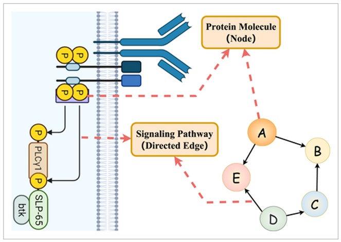
Figure 1. The structure of the causal protein signalling network.
In contemporary research, causal discovery methodologies have been successfully deployed across a wide range of biological networks [17], including causal protein signalling networks [18, 19], gene regulatory networks [20, 21], and brain effective connectivity networks [22, 23], among others. Matching the conventions of gene regulatory networks—another prevalent class of biological networks—the topology of a causal protein signalling network is regularly represented using a two-dimensional adjacency matrix. Nonetheless, these two biological network paradigms display fundamental discrepancies. A gene regulatory network maps out the control relationships governing gene expression, encapsulating transcriptional modulation mechanisms and the downstream impacts of transcription factors [24]. Consequently, research in that domain primarily probes the overarching logic and dynamics of gene expression control, alongside the regulatory deviations coupled with pathological states. Conversely, causal protein signalling networks are geared toward clarifying the operational routes of intracellular signal propagation and decoding the systemic modulation of cellular behavior and metabolic pathways mediated by direct protein-to-protein interactions.
Over recent years, a diverse array of methodologies has been formulated to deduce causal protein signalling networks. These analytical strategies can be broadly grouped into two main schools of thought, the first of which relies on classic machine learning paradigms. For instance, Sachs et al. [25] introduced a causal inference framework tailored for causal protein signalling networks using multiparameter single-cell datasets. This strategy allowed for a more precise determination of directional links within protein networks and produced a foundational bioinformatics benchmark dataset that remains extensively utilized in graphical modeling validation studies. Similarly, Zheng et al. [26] developed the NoTears formulation, which reframed the challenge of causal structure learning by shifting it from a discrete combinatorial optimization problem into a continuous optimization problem, thereby enabling more computationally efficient tracking of causal protein signalling paths. In another study, Zhang et al. [27] designed an approach for reconstructing causal protein signalling topologies directly from continuous observational profiles. Their framework implements a regression-based conditional independence test (RCIT) that merges kernel ridge regression (KRR) with the Hilbert-Schmidt independence criterion (HSIC) utilizing a permutation-based approximation. While this class of machine learning methods benefits from straightforward model architectures and fast execution speeds, the ultimate structural accuracy of the reconstructed causal protein signalling networks frequently leaves room for refinement.
The alternative paradigm centers on deep learning methodologies, which feature highly complex model architectures. Under this category, Löwe et al. [28] developed a novel framework termed amortized causal discovery (ACD), which exploits shared underlying dynamics across samples to accelerate the extraction of causal relationships from empirical data. Sanchez [29] introduced DiffAN, an identifiable discovery algorithm that utilizes a diffusion probabilistic model to establish a proper topological ordering, permitting causal network reconstruction under the structural assumptions of an additive noise model. Further advancing this domain, Zhu et al. [30] engineered a causal learning framework grounded in reinforcement learning (RL), deploying an RL agent to navigate and optimize candidate causal protein signalling network configurations. Additionally, Tristan et al. [31] presented a deep generative architecture that employs a flow-based network generation routine coupled with structural constraint variants to reconstruct causal protein signalling paths. While these deep learning-driven strategies can uncover causal protein signalling networks with higher topological accuracy, they typically generate substantial computational overhead and prolonged running times due to the parameterized complexity of their neural network backbones.
A Bayesian network is an unconstrained causal association framework that mathematically encodes the joint probability distribution governing a set of random variables within a specified domain [32]. A complete BN is defined by a specific graphical structure alongside a corresponding set of local conditional parameters [33]. The structural component is represented as a directed acyclic graph (DAG) that explicitly charts the causal dependencies connecting the domain variables.
The deployment of BN methodologies for mapping causal protein signalling networks has attracted substantial interest and yielded highly compelling outcomes. A core catalyst for its widespread adoption is the intrinsic capacity of BN frameworks to handle large scale node variables while executing structural searches across extensive spaces of candidate graph topologies. Consequently, numerous BN-oriented algorithms for identifying causal protein signalling paths have been brought forward recently. Chaturvedi et al. [34] proposed an innovative formulation combining BNs with extreme learning machines to reconstruct causal protein signalling networks. Zhou et al. [35] presented a hybrid strategy that fuses BNs with random forest classifiers to model and learn causal protein signalling pathways effectively. Adapting tools from engineering fields, Byun et al. [36] introduced a BN learning framework utilizing junction tree representations; though originally engineered for industrial system reliability assessments, this framework was successfully repurposed for the discovery of causal protein signalling architectures, highlighting its structural flexibility. Furthermore, Chobtham et al. [37] designed an advanced BN structure learning technique capable of accounting for latent variables, demonstrating strong performance when recovering complex, unobserved causal pathways within protein networks. Taken together, these studies underscore the rich variety and continuous evolution of BN-based frameworks within the domain of causal protein signalling network discovery, with each method offering unique analytical perspectives and technical advancements.
Nonetheless, these conventional methods often fail to exploit global search coordinates thoroughly, can suffer from severe computational complexity issues, and routinely ignore the cross-cell molecular interactions occurring across heterogeneous single-cell environments, which ultimately compromises the accuracy of the derived causal protein signalling graphs. To surmount these structural limitations, several strategies leveraging swarm intelligence metaheuristics to optimize BN graphs have been introduced in recent years. Ji et al. [38] formulated an ABC algorithm that uses a specialized scoring function to discover BN structures. Wang et al. [13] designed a discrete firefly optimization routine optimized for BN graph searches, while Fang et al. [14] developed a structure information-guided genetic algorithm (SIGA-BN) specifically tailored for learning BN configurations.
Among the aforementioned swarm intelligence approaches, the ABC metaheuristic is highly favored due to its streamlined algorithmic architecture, robust exploration traits, and pronounced search efficiency. A key characteristic of the ABC framework is its elegant integration of candidate solution construction and localized neighborhood searches into a unified metaheuristic loop: employed and onlooker bees execute local neighborhood explorations, while scout bees generate entirely new candidate solutions within the bounded feasible search space. Ji et al. [38] presented an extended ABC formulation that integrated the chemical signaling mechanisms characteristic of ant colonies into the ABC framework for the first time. The foundational premise of this extended ABC routine is that bees, much like ants, actively use chemical pheromones to modulate communication paths and steer collective behavior. Based on these flexible dynamics, ABC formulations have been successfully migrated to numerous optimization domains. For instance, Wang et al. [39] engineered a robust optimization framework combining krill herd logic with ABC principles and information exchange concepts, yielding high performance across various benchmark problems. Similarly, Wang et al. [40] coupled a localized information feedback model with the ABC search loop to substantially boost the convergence speed and performance of the algorithm. Finally, Liu et al. [41] introduced an ABC variant featuring dynamic penalty functions and Lévy flight mechanics, which significantly upgraded the algorithm's capacity for resolving tightly constrained optimization landscapes.
This section outlines the operational architecture of the newly developed parallel ABC framework (PDABC) designed for reconstructing causal protein signalling networks from single-cell repositories.
The proposed PDABC algorithm operates as a score-based optimization routine for training BNs within the context of causal protein signalling networks. It utilizes the discrete K2 score metric to orient its stochastic search toward the globally optimal network topology—defined as the specific BN graph configuration that achieves the maximum K2 score. Throughout this manuscript, the target causal protein signalling network is represented via a BN structure formalized as G = < Y, E >. The vertex set Y gathers all system coordinates, where each node a ∈ Y corresponds to a unique protein target or signaling component. The edge set E indexes the directed links, where each individual entry edgeab ∈ E charts a directed signalling dependency flowing from protein a to protein b. As a result, the challenge of mapping a causal protein signalling network reduces to estimating a valid BN structural topology from continuous or discrete single-cell measurements. The universal mathematical notations utilized throughout this paper are organized and defined in Table 1. A given BN uniquely characterizes and encodes the joint probability distribution across the entire set of domain variables Y = {Y1, Y2, Y3, ⋅⋅⋅Ym} according to the following factorization formula:
 (1)
Table 1. Explanations of the meaning of the universal notations.
Symbol / Notation | Description |
G | A Bayesian Network (BN) structure representing a causal protein signaling network. |
A | Single-cell dataset. |
g | Total number of cells. |
c | Total number of nodes. |
N | Number of parallel artificial bee colonies, equivalent to the number of sub-datasets. |
Gi(0), (1 ≤ i ≤ N) | Initial empty graph associated with the ith artificial bee colony. |
t | Current iteration index. |
NC | Predefined total number of iterations. |
D | Training dataset generated after discretizing A. |
K | Number of bees within a colony. |
k | Index of the kth bee in a colony. |
Gk(t) | Best solution associated with the kth bee during the tth iteration. |
Mi, (1 ≤ i ≤ N) | Pheromone matrix corresponding to the ith artificial bee colony. |
Bi | Best solution currently identified by the ith colony. |
Nk | Candidate solution obtained from a neighboring search. |
Pk(t) | Search process conducted by the kth bee during the tth iteration. |
thr | Maximum allowable number of mining attempts. |
Sk | Current mining count for the kth bee. |
GF | Combined adjacency matrix obtained after merging all results. |
G* | Final optimal causal protein signaling network. |
Single-cell data is represented as a two-dimensional matrix A consisting of c columns and g rows:
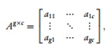 (2)
where aij (1 ≤ i ≤ g, 1 ≤ j ≤ c) denotes the expression value of the ith protein biomolecule within the jth single cell. Our objective is to reconstruct causal protein signalling networks utilizing these protein biomolecule expression profiles from single-cell data, thereby inferring directional signalling pathways between proteins to elucidate cellular signalling mechanisms.
The optimization target of PDABC is to maximize a network score, evaluated via the K2 metric in this study, which measures the likelihood of obtaining the observed dataset given a specific candidate network topology. The K2 metric is a standard scoring function applied during BN structural inference from discrete data matrices. It uses a Bayesian formulation to determine the joint probability of a BN structure. The baseline mathematical definition of the K2 metric is given by:
 (3)
where ri represents the number of discrete states available for the variable Yi, qi denotes the total number of unique parent state configurations within the parent set ∏(Yi), and Lijk counts the number of samples in the dataset D where the variable Yi takes its kth discrete value while its parent set ∏(Yi) matches its jth state configuration. Additionally,
 (4)
To arrive at an additively decomposable objective function, the natural logarithm of the baseline formulation is adopted as the practical K2 scoring metric, represented as T(G : D) rather than Q(G, D). Furthermore, assuming a uniform prior distribution across all candidate network topologies, the constant term log Q(G) can be omitted from consideration, as detailed in [42]. Consequently, the simplified metric T(G : D), which rates the performance of a network topology G relative to a training dataset D, can be decomposed as shown in Eq. 4:
In Eq. 4, the component T (Yi, ∏ (Yi)) signifies the local K2 scoring contribution computed for each individual vertex within the graph G. Its formal algebraic definition is expressed as:
 (5)
Eq. 5 establishes that the local K2 score contribution of any given node is governed exclusively by its immediate local parent structure. Because joint probabilities scale between 0 and 1, computing the K2 metric via log(Q(G, D)) consistently generates a negative numerical value. The K2 metric can be formalized using either Q(G, D) or \log(Q(G, D)). Accordingly, the largest K2 numerical value identifies the optimal BN graph configuration. The objective function seeks to maximize this aggregate K2 metric by varying the binary entries of Yij to uncover the superior network topology. Furthermore, the estimated causal protein signalling network must fulfill the following formal structural constraints:
Causal Constraints: For any pair of proteins Yi and Yj, the causal link is bound by the condition that Yij = 1 denotes the existence of a directed causal connection pointing from Yij This constraint establishes and enforces edge directionality throughout the network.
Acyclic Constraints: To guarantee that the inferred network is a valid directed acyclic graph (containing no loops), supplementary topological constraints are enforced to prevent cycle formation. This is achieved by ensuring that no directed sequence of edges permits a path to connect a protein back to itself.
The functional pipeline of the PDABC algorithm is structured around three sequential phases: discretization and initialization, parallel ABC search, and information fusion. More specifically, during the discretization and initialization phase, the continuous single-cell values are first converted into three discrete categorical levels; following this, the framework instantiates an empty graph structure along with a pheromone matrix for each sub-colony, which are utilized to assemble candidate solutions and log pheromone variations throughout the exploration process, respectively. Throughout the parallel colony search phase, N independent artificial bee colonies execute optimization sweeps across different datasets concurrently. Each parallel sub-colony maintains three distinct agent roles: employed bees, onlooker bees, and scout bees. Once the employed bees conclude their localized neighborhood structures searches, they transmit their solution metrics to the onlooker bees. The onlooker bees then proceed with further neighborhood searches after selecting their target solutions according to a probability distribution. If a candidate solution fails to show any fitness improvement over a pre-specified number of continuous iterations, the corresponding employed bees transition into scout bees to initialize a search for entirely new solutions. During the subsequent information fusion phase, as soon as all sub-colonies complete an identical epoch, the localized pheromone profiles from all groups are combined and averaged to establish the baseline pheromone state for the next generation, steering the swarm's exploration paths in the upcoming iteration. Upon completing the maximum pre-established iteration count NC, the N optimal graphs tracked by each sub-colony are compiled into a master adjacency matrix G, and the single final causal protein signalling network is resolved according to specific extraction rules. Figure 2 charts the complete flowchart of the PDABC method.
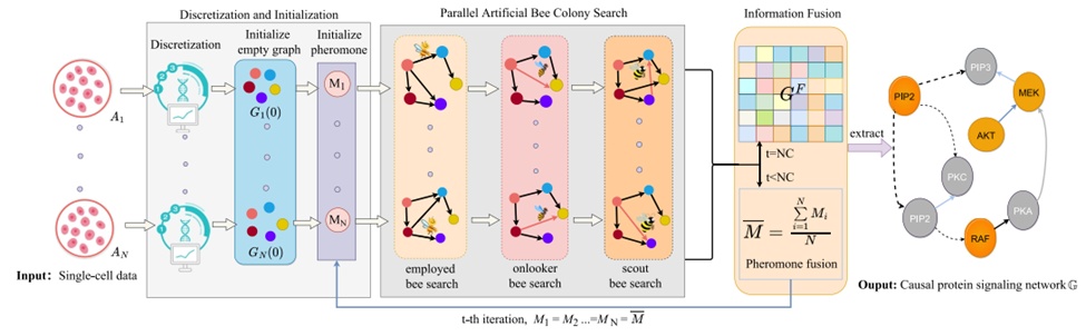
Figure 2. The flowchart of the PDABC algorithm. The PDABC algorithm consists of three main phases. The discretisation and initialisation phase includes the discretisation of single-cell data and the initialisation of empty graphs and pheromones. Parallel artificial bee colony search phase includes employed, onlooker, and scout bee search processes. Information fusion includes pheromone fusion and the fusion of the learnt causal protein signalling networks. PDABC, parallel discrete artificial bee colony.
In line with numerous score-based BN learning formulations, PDABC incorporates the K2 scoring metric. Because this evaluation function cannot directly process continuous variables, data discretization is a mandatory preliminary step. During initial data cleaning, outlier measurements that deviate from the sample mean by more than three standard deviations are filtered out. Next, the remaining continuous values are mapped into three discrete categories corresponding to high, medium, or low activation levels of the phosphorylated protein target. This discretization scheme utilizes an agglomerative technique designed to minimize the reduction of pairwise mutual information across the system variables. Through this method, the data points are structured for subsequent computational exploration and biological interpretation. For data collected under specific chemical perturbations, the values for all vertices within each single-cell matrix can be parsed into three distinct groups. Operationally, the data entries within each column of matrix A are first sorted in ascending order, and the number of data points allocated to each discrete interval, denoted as len, is calculated as follows:
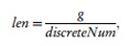 (6)
where discreteNum is assigned a constant value of 3. Utilizing this interval size, the boundaries for the frequency thresholds ei are defined according to the following set relation:
 (7)
where min represents the minimum value identified within that specific data column. Ultimately, the continuous raw measurements are mapped to their corresponding discrete values one by one based on these interval boundaries. This divides the dataset into three equal-sized blocks for each protein target. These protein expression values are categorized into three distinct operational states: high (assigned value = 3), medium (assigned value= 2), and low (assigned value= 1). Each of these three segments accounts for roughly 33.33% of the total recorded data points, ensuring a uniform distribution across the discrete protein expression categories. This systematic partitioning enforces a balanced representation of the biological data for subsequent network inference and structural modeling.
During the initialisation stage of the PDABC algorithm, specific parameters must be assigned their starting values. To begin, N separate artificial bee colonies are created. Each colony is configured with a size of K and contains K individual bees to execute parallel searches across N single-cell datasets. Within the context of PDABC, food source locations represent potential solutions to the problem. Consequently, N empty graphs Gi(0) (1 ≤ i ≤ N) containing identical sets of nodes are initialised across the N colonies, serving as the initial food source for each respective colony. The maximum allowable iterations are restricted by the parameter NC. Furthermore, to ensure bees do not become trapped in infinite loops while exploiting a specific food source, a maximum mining threshold is established via the parameter thr. Additionally, within each separate colony, bees generate pheromones as they navigate, using these chemical paths to share information regarding food sources. Throughout the construction of a candidate solution, every bee originates from a designated starting node and sequentially identifies valid adjacent nodes. During this routine, pheromones progressively decay over time, leaving specific traces. As a result, a c-dimensional pheromone matrix M must be initialised for each separate colony to document pheromone dynamics throughout the search. In this study, c denotes the total node count within graph G, which corresponds directly to the dimensionality of the input data. The PDABC algorithm incorporates the K2 metric to evaluate the quality of generated solutions and to direct the optimization routine during graph construction.
In this segment, the PDABC framework concurrently deploys N distinct colonies across N datasets to perform a parallelised search for causal protein signalling networks that optimize the K2 metric. drawing upon the concepts presented by [38] indicating that bees possess communication pathways analogous to ants, the optimal solution for each of the N colonies is derived through the following recurrent procedure: every individual bee, designated as k, starts its search with an empty graph Gi(0), where 1 ≤ i ≤ N. The bee progressively develops connected solutions by introducing a single edge at each step until the structure achieves its maximal score. The selection of a directed edge from the available runtime candidate edges at time t is governed by a probabilistic transition rule formulated as:
 (8)
where ζij(t) denotes the current pheromone density, β represents a weighting coefficient regulating the impact of Γij(t) on the selection of edges, and Γij(t) signifies the heuristic information associated with edge bi,j. The set HXk(t) encompasses all prospective candidate edges exhibiting positive heuristic values. The parameter q_0 (where 0 ≤ q0 < 1) defines the baseline balance between exploration and exploitation. The random variable q is uniformly drawn from the continuous interval [0, 1]. Ultimately, a node pair I and J is chosen stochastically in accordance with the following probability function:
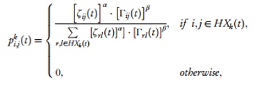 (9)
where α denotes the relative weight assigned to the pheromone concentration ζrl(t) deposited by companion bees. The heuristic function Γij is formalised as follows:
 (10)
As illustrated in Figure 2, the optimization routine for each individual colony is segregated into three distinct phases: the employed bee search, the onlooker bee search, and the scout bee search.
Initially, each employed bee is assigned a null solution structure. It subsequently searches for a modified configuration featuring an enhanced K2 metric relative to the baseline solution within its immediate structural neighbourhood. This is achieved by evaluating and executing four fundamental evolutionary operators, defined as follows:
Add: Two distinct nodes, Yi and Yj, are chosen at random such that i ≠ j and Yi ∈ Y \ ∏ (Yj). Provided that the introduction of edge bij = Yi → Yj does not induce a directed cycle, the updated solution is generated by incorporating this edge into the current topology: Gh+1 = Gh ∪ {bij}.
Delete: This operator stochastically targets an existing edge bij within the graph Gh, where Yj represents the child node and Yj signifies the parent node. The designated edge is subsequently extracted from the structure, yielding a modified solution: Gh−1 = Gh\{bij}.
Reverse: This operator randomly targets an edge bij within the graph Gh and inverts its orientation, provided that this inversion does not introduce a directed cycle. The updated solution is achieved by purging the edge bij from the graph and inserting the inverted edge bji: = Gh \ bij ∪ {bji}
Move: This operator targets nodes Yi and Yi that possess non-empty parent sets. The operator selects one parent node for Yi and one for Yi, designated as Yk ∈ ∏ (Yi) and Yl ∈ ∏ (Yj), where k ≠ l. If the conditions Yl ∈ (Y \ (∏(Yi) ∪ {Yi})) and Yk ∈ (Y \ (∏(Yj) ∪ {Yj})) are met, and the adjustment maintains a valid DAG structure, the parent configurations for both nodes are altered concurrently. This procedure yields an updated solution featuring modified parent allocations.
Figure 3 illustrates these four baseline evolutionary operators acting upon an employed bee solution Gh. Once all employed bees conclude their local neighborhood operations, they communicate their structural solutions to the onlooker bees. The onlookers select their preferred solution based on a probability distribution defined as:
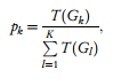 (11)
where T(Gk)represents the calculated K2 metric score of the Bayesian Network structure k, and K denotes the total number of candidate solutions.
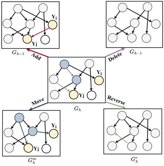
Figure 3. The four basic evolution operators of a solution G_h for employed bees.
Utilising Eq. 11, a roulette wheel selection scheme is applied to allocate food sources to the onlooker bees. Within this selection framework, the likelihood of choosing a specific solution is directly proportional to its computed K2 score. Consequently, structures exhibiting higher K2 metrics possess a greater probability of selection, rendering them more appealing to onlooker bees than lower-scoring alternatives.
Following solution selection, the onlooker bee advances into its respective neighbourhood search phase. Here, each onlooker bee can implement the four baseline evolutionary operators alongside two specialized knowledge-driven operators to isolate an optimal configuration with an elevated K2 metric. In this study, the optimal configuration identifies the targeted coordinates for the subsequent deployment of the employed bee. The two knowledge-driven operators are detailed as follows:
KD_Addition: This operator serves as an advanced variant of the previously defined Add operator. When determining the insertion of a new edge into the active solution Gh, it evaluates the recorded K2 metrics of edges missing from Gh. Missing edges featuring higher K2 values are granted a higher probability of selection. This strategic preference relies on the property that the global K2 metric of a causal protein signalling network is decomposable into individual variable scores. The objective of the algorithm is to discover a causal protein signalling network that maximises the overall K2 metric. When inserting an edge from a given node to Yi, prioritizing an edge with an elevated K2 metric is preferred, as it is more likely to improve the local K2 metric T (Yi, ∏ (Yi)) of node Yi.
KD_Deletion: This operator functions as an advanced variant of the previously defined Delete operator. When the mechanism determines that an existing edge within the active solution Gh should be purged, it references the recorded K2 metrics of all current edges in Gh. Edges demonstrating lower K2 values are targeted for removal with higher probabilities. This operational bias is designed to minimise the reduction in the local K2 metric of node Yi. By prioritizing the elimination of low-scoring K2 edges, the framework aims to mitigate potential drops in the K2 score of node Yi.
If a candidate solution fails to show improvement for thr consecutive iterations, indicating that the fitness level of the food source has reached a plateau, the solution is assumed to have converged to a local optimum. In this scenario, the employed bee abandons this specific food source and transitions into a scout bee. The scout bee then constructs a brand-new solution by leveraging the existing pheromone tracks and heuristic data remaining on the edges. Following this reconstruction, the scout bee reverts to an employed bee to resume the optimization process. Once the updated statuses of all solutions from the employed bees are established, the top-performing solution represents the optimal causal protein signalling network discovered by that specific colony during its search on the corresponding dataset.
Let (1≤ i ≤ N) denote the optimal solution discovered up to the current iteration across the N colonies, and let T ( : D) represent the metric score of this optimal solution for the i-th population search. At this juncture, the pheromone concentrations ζij(t) are updated to retain the structural information of the optimal solutions identified during the current iteration for each of the N bee colonies. The update rule is formulated as:
 (12)
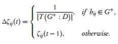 (13)
The aforementioned search routine is executed concurrently by N independent colonies. Upon completion of this process by all N colonies, the pheromone matrices from M1 to MN are updated using the pheromone configurations of the best solution. This marks the conclusion of the current iteration's search phase, and the algorithm transitions into the information fusion phase.
This section introduces a novel information fusion mechanism structured into two distinct stages: pheromone fusion and causal protein signalling network extraction. Figure 4 illustrates the detailed sequence for extracting the final causal protein signalling network.
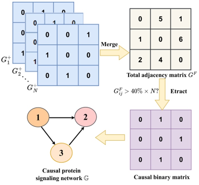
Figure 4. The detailed process of extracting the final causal protein signalling network.
In detail, when the parallel artificial bee colony search finishes, if the current iteration count t is less than NC, all bee colonies initiate pheromone fusion according to the following mathematical rule:
 (14)
where represents the consensus average matrix computed from the pheromone matrices of the N colonies. Following this fusion, all pheromone matrices from M1 to MN associated with the N colonies and their current optimal solutions are updated to match this average pheromone matrix. This consensus matrix serves as the initial pheromone distribution for the subsequent iteration, guiding each colony in its ongoing search for the optimal causal protein signalling network. When the iteration counter t reaches the threshold NC, the iterative loop terminates. The algorithm then enters the causal protein signalling network extraction phase, where the N optimal solutions to generated in parallel by the N colonies are merged. Each individual solution is represented as an adjacency matrix, and these N matrices are summed into a cumulative adjacency matrix GF. An extraction threshold rule is then applied to GF: if an entry within GF exceeds 40\% of N, the entry is set to 1; otherwise, it is reset to 0. Through this filtering, the final causal protein signalling network is established.
In summary, the proposed PDABC algorithm is structured into three primary phases: (1) discretisation and initialisation, (2) parallel artificial bee colony search, and (3) information fusion. The comprehensive procedure is outlined in Algorithm 1.
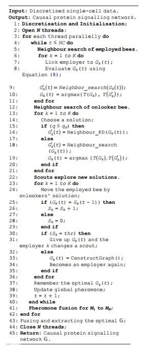
Algorithm 1. PDABC
For the discretisation and initialisation phase, the PDABC algorithm first initialises N separate colonies and allocates N concurrent computational threads for them. Subsequently, PDABC generates an initial set of empty graphs Gi(0) (1 ≤ i ≤ N) and configures the baseline parameters for each individual colony. Finally, N single-cell datasets are discretised and fed as input into the algorithm.
During the parallel artificial bee colony search phase, solution (food source) quality is appraised via the K2 metric. The PDABC framework utilizes three categories of bees for neighbourhood exploration: employed bees, onlooker bees, and scout bees. Within each individual iteration, employed bees first construct solutions with superior K2 metrics by evaluating and executing four baseline evolutionary operators, moving to the newly discovered topology if it yields a higher score. Once all employed bees complete these steps, they share their structural solution data with the onlookers. Onlooker bees then choose a preferred solution based on the probability distribution defined in Eq. 11, exploring for higher K2 metrics by executing the four baseline evolutionary operators alongside two knowledge-driven operators. If a solution tracked by the employed bees stalls without improvement for a predetermined number of iterations thr, the employed bee abandons that site and transitions into a scout bee. Leveraging the heuristic details and the remaining edge pheromones, the scout bee reconstructs a new solution topology and reverts back to an employed bee. This iteration's search phase concludes when the scout bees across all N colonies have established their final solutions.
During the information fusion phase at the conclusion of each iteration, the pheromones across all colonies are consolidated. Post-fusion, the pheromone matrix of every individual colony is synchronized to the average of all pheromone matrices, serving as the baseline pheromone state for the next iteration to guide the colonies toward optimal causal protein signalling networks. When the iteration counter t reaches the predefined maximum limit NC, the N optimal solutions to from the N colonies are summed into a global composite solution GF . Finally, the definitive causal protein signalling network is extracted from GF using the designated percentage threshold rule. At this stage, the N active computational threads are terminated, and the algorithm concludes execution.
Based on the operational details of Algorithm 1, the computational complexity of PDABC can be evaluated as follows: let the system ingest N distinct datasets, let NC denote the maximum iteration count, and let K represent the number of bees allocated per colony. The time complexity of the PDABC algorithm can be formalised as O(NC) ⋅ O(3K + N) ≈ O(n2). In contrast, the time complexity of a non-parallel discrete artificial bee colony (DABC) approach is formulated as O(N) ⋅ O(NC) ⋅ O(3K) ≈ O(n3). Evidently, PDABC introduces an additional computational overhead of O(N) primarily during the pheromone fusion stage when compared to DABC; however, when resolving protein networks across multiple datasets, the total execution time of PDABC is significantly lower than that of DABC. This performance advantage becomes increasingly pronounced as the total number of datasets N scales up.
This section presents experimental evaluations conducted on simulated datasets to appraise the performance of the PDABC algorithm and contrast its capabilities with alternative state-of-the-art frameworks. Furthermore, the practical utility of PDABC is showcased by applying the method to a previously open-sourced multi-parameter FACS dataset, thereby validating and illustrating its operational efficacy. The benchmarking hardware platform consists of a personal computer configured with an Intel Core i5-8300 processor, 16 GB of RAM, a 2.30 GHz CPU, running a Windows 10 operating system. The PDABC algorithm is compiled and executed in Java using the Eclipse integrated development environment running JDK version 1.8.
The methodology for constructing the simulated datasets is summarized below. For a more comprehensive breakdown of this framework, please see the reference study [30]. The synthesis of the simulation datasets depends on a designated number of variables, denoted as v, for which a h × h upper triangular matrix is established to serve as the adjacency matrix of a directed acyclic graph. The upper entries of this matrix are stochastically sampled from a Bernoulli distribution featuring a success probability of 0.5. To populate the edge weights, values are independently drawn from a uniform distribution spanning the intervals [-1.5, -0.5] ∪ [0.5, 1.5], yielding a composite weight matrix F ∈ ℝ h × h. Following this, a noisy signal matrix O is generated via the linear transformation:
o = FTo + γ
where γ represents the error term. This noise factor can be modeled using either a Gaussian or a non-Gaussian distribution. A unit noise variance is selected for both models, and a sample size of m = 200 is designated for each sub-dataset. The variables are subsequently arranged in a random sequence. Ultimately, ten distinct simulation datasets, labeled sim1 through sim10, are constructed. Each individual simulation dataset features a varying number of nodes (v = 5, 10, 20, 30, 50) and is arranged in sequence with a varying number of sub-datasets (N = 10, 50). Within the PDABC architecture, the input allocated to each individual colony corresponds to a single sub-dataset from a given simulation dataset, whereas the baseline comparison algorithms ingest the entire simulation dataset as a single unified input.
In this study, empirical multi-parameter fluorescence-activated cell sorting data [25] are leveraged to deduce directional protein signalling pathways from the expression profiles of target proteins and phospholipids. The underlying FACS data repositories are accessible at https://www.science.org/doi/10.1126/science.1105809#supplementary. This specific bioinformatics resource is widely deployed as a benchmark for evaluating graphical network configurations in molecular biology. The dataset aggregates experimental annotations and supplies continuous measurements reflecting the expression dynamics of numerous phosphorylated proteins and phospholipid components within human immune cells. Furthermore, the dataset outlines a theoretical network model that establishes the sequential dependencies among pathway constituents. It comprises 11 distinct signalling nodes, where each node represents an individual phosphorylated protein molecule active within the primary human T-cell transduction pathway. Over the past two decades, a combination of classical biochemical assays and genetic analyses has validated a causal protein architecture that serves as the ground-truth benchmark. This validated gold-standard network possesses 17 high-confidence causal arcs. The compilation is partitioned into 14 distinct sub-datasets that correspond to 14 independent biochemical perturbations. The sample size within each sub-dataset spans from 723 to 917 observations, with each sub-cohort subjected to unique experimental perturbations, as detailed in Table 2. Prior to analysis, all data segments are discretised according to the methodology.
Table 2. Description of each sub-dataset in FACS dataset.
Dataset | Size | Stimulation |
1 | 853 | CD28, CD3 |
2 | 902 | ICAM-2, CD28 |
3 | 911 | CD28, CD3, akt-inhibitor |
4 | 723 | CD28, CD3, G0076 |
5 | 810 | CD28, CD3, Psitectorigenin |
6 | 799 | CD28, CD3, U0126 |
7 | 848 | CD28, CD3, LY294002 |
8 | 913 | PMA |
9 | 707 | β2camp |
10 | 899 | ICAM-2, CD28, CD3, akt-inhib |
11 | 753 | ICAM-2, CD28, CD3, G0076 |
12 | 868 | ICAM-2, CD28, CD3, Psitectorigenin |
13 | 759 | ICAM-2, CD28, CD3, U0126 |
14 | 927 | ICAM-2, CD28, CD3, LY294002 |
The topological structures of the inferred protein networks are validated against the ground-truth causal graphs using six standard network assessment criteria: (1) Precision; (2) Recall; (3) F1; (4) Accuracy; (5) Structural Hamming Distance (SHD); and (6) Time. Formally, the metrics of Precision, Recall, and F1 are expressed as follows:
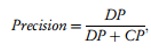 (15)
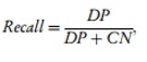 (16)
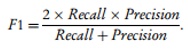 (17)
In this analytical framework, DP represents the total count of true positive arcs, where an arc denotes a directed connection between paired nodes. Conversely, CP signifies the total count of false positive arcs, DN indicates the count of true negative non-edges, and CN represents the count of false negative arcs. Consequently, the operational limits of both Recall and Precision scale between 0 and 1, with the F1 score representing their harmonic mean. These performance indices offer a multidimensional validation of the model's capacity to correctly resolve authentic positive interactions while simultaneously suppressing both type I and type II errors.
As an omnibus structural assessment metric, Accuracy is defined as follows:
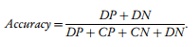 (18)
The SHD metric quantifies the absolute number of elementary structural modifications required to align the learned causal network topology with the ground-truth graph. It yields a discrete measure of the distance between the reconstructed model and the true biological path, thereby indicating how effectively the learning mechanism isolates the underlying dependencies among proteins.
Concretely, the SHD aggregates the cumulative edge deletions, insertions, and orientation reversals required to map the estimated network topology precisely onto the ground-truth graph. The SHD value is derived using the following formulation:
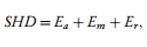 (19)
where Ea denotes the quantity of redundant edges requiring removal, Em marks the number of omitted edges requiring insertion, and Er represents the count of inverted edges requiring a reversal of directionality. Finally, the total execution duration of the algorithm, measured in seconds, is captured by the Time index.
To benchmark the performance of the proposed PDABC framework against current paradigms, its efficiency is contrasted with seven state-of-the-art or classic structural learning algorithms. This comparative baseline includes: continuous optimisation for structure learning (NoTears) [26], RL [30], PC [8], GES [11], DAG structure learning with graph neural networks (DAG-GNN) [43], diffusion models for causal discovery via topological ordering (DiffAN) [29], and a novel framework for ACD [28]. Additionally, to verify whether the parallelized design mitigates computational bottlenecking and whether the information fusion mechanism enhances network reconstruction accuracy, ablation trials are introduced. These trials benchmark PDABC against a localized, non-parallel ABC variant (DABC) that omits the inter-colony pheromone and structural fusion stages.
The operational parameters governing the baseline models are initialized in strict accordance with their original source publications. To establish an equitable benchmarking environment, validation is conducted on synthetic datasets containing between 5 and 50 nodes, with fine-tuning applied to the baseline parameters to ensure that all comparison models operate at peak capacity.
The hyper-parameter profile of PDABC encompasses the pheromone trail sensitivity (α), the heuristic information weight (β), the pheromone decay rate (ρ), the exploitation-exploration balance index (q0), the maximum iteration threshold (NC), and the total agent population per colony (K). Following comprehensive empirical tuning, the configuration of α = 1.8, β = 1.8, ρ = 0.15, and q_0 = 1.5 was found to yield optimal robustness across the majority of synthetic datasets. Meanwhile, the parameters NC and K primarily govern structural stability and convergence trajectories. Consequently, sensitivity experiments were performed on simulated data to determine the ideal settings for these two parameters within PDABC. It was observed that scaling NC and K monotonically enhanced the structural resolution of PDABC at the expense of computational duration; the algorithm achieved peak topological accuracy and asymptotic stability at NC = 10 and K = 20, establishing the final operational parameters. Throughout all simulation trials, a strict control variate protocol was enforced, whereby individual parameters were isolated and modulated while maintaining all other variables static. The complete parameter allocations for all nine frameworks are summarized in Table 3.
Table 3. Parameter settings of 9 algorithms.
Algorithms | Parameters |
NoTears [26] | λ1 = 0.1, maxiter = 100, threshold = 0.3 |
RL [30] | epoch = 50, α = 0.99 |
PC [8] | α = 0.05 |
GES [11] | k = 0.01, N = 10 |
DAG-GNN [43] | epoch = 250, η = 10, γ = 1 |
DiffAN [29] | epoch = 300, nsteps = 100 |
ACD [28] | epoch = 500, γ = 0.5 |
DABC | α = 1.8, β = 1.8, ρ = 0.15, q0 = 1.5 |
NC = 10, K = 20, discreteNum = 3 | |
PDABC | α = 1.8, β = 1.8, ρ = 0.15, q0 = 1.5 |
NC = 10, K = 20, discreteNum = 3 |
The initial comparative validation of PDABC against the eight alternative frameworks is conducted using 10 distinct synthetic datasets. Following this evaluation of algorithmic capacity and accuracy, benchmarking is extended to the real-world FACS repositories. Notably, all algorithms undergo 10 independent execution cycles across both synthetic and empirical data, with the arithmetic mean reported as the definitive result. When executing PDABC, the N sub-datasets are distributed concurrently to the respective N parallel artificial bee colonies. For the baseline frameworks, the individual sub-datasets must be concatenated into a single, unified matrix to serve as the input vector. For stochastic optimization paradigms, structural variance and stability are illustrated by presenting the results in the form of mean \pm standard deviation. Lastly, because DABC and PDABC utilize the K2 scoring metric, the input datasets are subjected to a mandatory preliminary discretisation step.
A comprehensive empirical comparison of the nine algorithms is executed using the 10 synthetic datasets, each defined by a specific node dimensionality c and a variable sub-dataset count N. Six graph evaluation metrics—Precision, Recall, F1, Accuracy, SHD, and Time—are tracked to quantify the performance profiles of the competing frameworks. A superior architectural model is characterized by elevated values for Precision, Recall, F1, and Accuracy, coupled with minimized values for both SHD and execution Time. The granular data derived from these 10 simulation datasets are detailed in Table 4. Within this table, bold typeface indicates that the corresponding algorithm achieved top-tier performance for that specific evaluation index.
Table 4. Comparisons of 9 algorithms on 10 simulation datasets.
Dataset (c, N) | Evaluation Measure | PDABC | DABC | ACD | DiffAN | DAG-GNN | GES | PC | RL | NoTears |
Sim1 (5, 10) | Precision Score | 0.78 ± 0.01 | 0.57 ± 0.03 | 0.37 ± 0.03 | 0.38 ± 0.04 | 0.33 | 0.57 | 0.50 | 0.60 | 0.61 |
Recall Score | 0.78 ± 0.01 | 0.62 ± 0.02 | 0.50 ± 0.02 | 0.27 ± 0.03 | 0.33 | 0.33 | 0.50 | 0.50 | 0.66 | |
F1 Measure | 0.78 ± 0.01 | 0.59 ± 0.02 | 0.42 ± 0.02 | 0.32 ± 0.02 | 0.33 | 0.42 | 0.50 | 0.54 | 0.64 | |
Classification Accuracy | 0.86 ± 0.01 | 0.81 ± 0.03 | 0.76 ± 0.02 | 0.74 ± 0.03 | 0.75 | 0.76 | 0.78 | 0.81 | 0.83 | |
Structural Hamming Distance (SHD) | 2.15 ± 0.52 | 4.40 ± 0.85 | 4.12 ± 0.65 | 7.15 ± 0.95 | 4.00 | 4.00 | 5.00 | 5.00 | 3.00 | |
Runtime (s) | 0.42 ± 0.01 | 0.79 ± 0.04 | 44.98 ± 0.88 | 47.59 ± 0.59 | 20.90 | 5.62 | 2.12 | 13.60 | 2.56 | |
Sim2 (5, 50) | Precision Score | 0.75 ± 0.01 | 0.60 ± 0.02 | 0.51 ± 0.04 | 0.42 ± 0.06 | 0.36 | 0.55 | 0.50 | 0.50 | 0.45 |
Recall Score | 0.77 ± 0.01 | 0.35 ± 0.02 | 0.61 ± 0.03 | 0.35 ± 0.06 | 0.29 | 0.35 | 0.23 | 0.50 | 0.52 | |
F1 Measure | 0.76 ± 0.01 | 0.44 ± 0.02 | 0.55 ± 0.04 | 0.38 ± 0.06 | 0.32 | 0.43 | 0.31 | 0.50 | 0.48 | |
Classification Accuracy | 0.83 ± 0.02 | 0.78 ± 0.02 | 0.77 ± 0.03 | 0.70 ± 0.04 | 0.73 | 0.75 | 0.73 | 0.81 | 0.78 | |
Structural Hamming Distance (SHD) | 2.11 ± 0.50 | 4.21 ± 1.25 | 3.25 ± 0.52 | 6.15 ± 0.89 | 7.00 | 5.00 | 6.00 | 3.00 | 4.00 | |
Runtime (s) | 0.58 ± 0.03 | 1.60 ± 0.09 | 53.37 ± 1.52 | 53.90 ± 1.34 | 30.90 | 10.69 | 3.40 | 25.62 | 3.80 | |
Sim3 (10, 10) | Precision Score | 0.76 ± 0.01 | 0.50 ± 0.02 | 0.54 ± 0.04 | 0.58 ± 0.04 | 0.63 | 0.47 | 0.64 | 0.71 | 0.54 |
Recall Score | 0.72 ± 0.01 | 0.59 ± 0.01 | 0.29 ± 0.02 | 0.65 ± 0.05 | 0.66 | 0.44 | 0.50 | 0.66 | 0.56 | |
F1 Measure | 0.74 ± 0.01 | 0.54 ± 0.02 | 0.37 ± 0.03 | 0.62 ± 0.04 | 0.65 | 0.46 | 0.56 | 0.68 | 0.55 | |
Classification Accuracy | 0.86 ± 0.01 | 0.81 ± 0.02 | 0.74 ± 0.05 | 0.81 ± 0.04 | 0.79 | 0.79 | 0.76 | 0.82 | 0.80 | |
Structural Hamming Distance (SHD) | 6.15 ± 1.85 | 9.21 ± 2.45 | 11.65 ± 0.85 | 9.15 ± 0.91 | 8.00 | 11.00 | 9.00 | 8.00 | 9.00 | |
Runtime (s) | 0.62 ± 0.01 | 1.49 ± 0.03 | 62.89 ± 0.16 | 59.20 ± 0.23 | 32.60 | 9.87 | 3.23 | 20.02 | 3.72 | |
Sim4 (10, 50) | Precision Score | 0.75 ± 0.01 | 0.53 ± 0.03 | 0.54 ± 0.06 | 0.47 ± 0.11 | 0.50 | 0.50 | 0.52 | 0.50 | 0.62 |
Recall Score | 0.73 ± 0.02 | 0.53 ± 0.02 | 0.50 ± 0.07 | 0.49 ± 0.09 | 0.30 | 0.50 | 0.60 | 0.59 | 0.62 | |
F1 Measure | 0.74 ± 0.02 | 0.53 ± 0.03 | 0.52 ± 0.06 | 0.48 ± 0.10 | 0.40 | 0.50 | 0.52 | 0.54 | 0.62 | |
Classification Accuracy | 0.88 ± 0.01 | 0.83 ± 0.02 | 0.79 ± 0.04 | 0.78 ± 0.05 | 0.76 | 0.80 | 0.83 | 0.83 | 0.84 | |
Structural Hamming Distance (SHD) | 5.55 ± 0.95 | 9.25 ± 2.50 | 9.03 ± 1.14 | 10.15 ± 1.02 | 11.00 | 10.00 | 9.00 | 9.00 | 8.00 | |
Runtime (s) | 1.56 ± 0.12 | 4.90 ± 0.15 | 63.65 ± 2.42 | 68.67 ± 1.32 | 54.60 | 13.76 | 3.97 | 30.30 | 4.23 | |
Sim5 (20, 10) | Precision Score | 0.80 ± 0.01 | 0.45 ± 0.02 | 0.79 ± 0.03 | 0.60 ± 0.04 | 0.51 | 0.31 | 0.40 | 0.54 | 0.53 |
Recall Score | 0.57 ± 0.01 | 0.43 ± 0.02 | 0.19 ± 0.03 | 0.14 ± 0.03 | 0.53 | 0.47 | 0.47 | 0.29 | 0.53 | |
F1 Measure | 0.67 ± 0.01 | 0.44 ± 0.02 | 0.31 ± 0.03 | 0.23 ± 0.03 | 0.52 | 0.37 | 0.43 | 0.37 | 0.53 | |
Classification Accuracy | 0.89 ± 0.02 | 0.77 ± 0.03 | 0.76 ± 0.03 | 0.78 ± 0.04 | 0.77 | 0.78 | 0.74 | 0.78 | 0.80 | |
Structural Hamming Distance (SHD) | 9.25 ± 0.55 | 14.15 ± 0.95 | 17.02 ± 1.56 | 19.15 ± 1.12 | 14.00 | 19.00 | 21.00 | 16.00 | 14.00 | |
Runtime (s) | 2.42 ± 0.28 | 5.22 ± 0.35 | 71.24 ± 1.39 | 73.37 ± 1.12 | 50.10 | 15.65 | 4.25 | 27.51 | 4.21 |
Note: The bold values indicate that the algorithm achieved the best results.
As evidenced by Table 4, PDABC consistently surpasses the alternative 8 frameworks across all evaluation metrics when tested on the 10 simulation datasets. This optimization advantage is distinct when tracing the two data trajectories: Sim1-Sim3-Sim5-Sim7-Sim9 and Sim2-Sim4-Sim6-Sim8-Sim10. Each distinct pathway comprises 5 datasets characterized by an incrementally scaling node dimensionality, specifically featuring 5, 10, 20, 30, and 50 nodes, respectively. The structural variance between these two trajectories lies in the sub-dataset density: every dataset in the primary trajectory aggregates 10 sub-datasets, whereas each configuration in the secondary trajectory integrates 50 sub-datasets. Observation indicates that across both pathways, the F1 scores of all evaluated models, including PDABC, undergo a marginal contraction while execution durations lengthen as the node count increases. Nevertheless, the accuracy metrics of PDABC experience less degradation under high node dimensions compared to baseline architectures, while its computational footprint exhibits the smallest increase. At the highest dimensionality of 50 nodes, PDABC maintains commanding F1 scores of 0.63 and 0.67 on Sim9 and Sim10, requiring merely 5.27 and 5.76 s, respectively; this performance substantially eclipses alternative frameworks and preserves peak topological accuracy.
To provide a more explicit visual diagnostic of algorithmic variance, the mean performance profiles of the 9 methods across the 10 simulation datasets are aggregated into a box plot, presented in Figure 5. These experimental trends reinforce that our proposed methodology yields highly stable distribution profiles across all targeted evaluation criteria, alongside a major improvement in execution latency and network mapping precision relative to contemporary models. The subsequent section extends this evaluation to real-world FACS single-cell datasets.
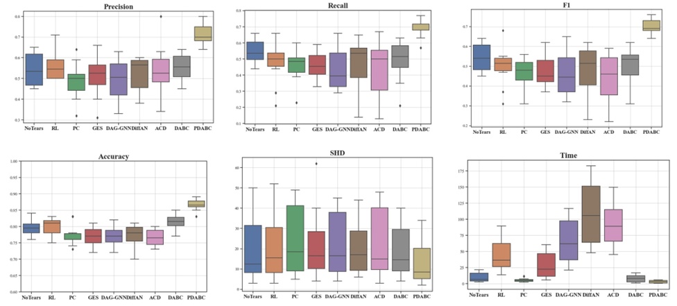
Figure 5. The average results of 9 algorithms are depicted on 10 simulation datasets, with each algorithm evaluated based on 6 metrics. The box plot illustrates the middle 50% of the data, with a horizontal line within the box indicating the mean value. The horizontal axis represents the 9 algorithms, while the vertical axis represents the values of the evaluation metrics.
In this section, the performance of PDABC is scrutinized using six key graph validation criteria—Precision, Recall, F1, Accuracy, SHD, and Time—to deduce causal protein signaling pathways from empirical FACS single-cell matrices. Initially, to evaluate the structural fidelity of PDABC across varying sample densities, the first 200, 400, and 600 observations are sequentially isolated from the 14 baseline sub-datasets to assemble three composite datasets with sample dimensions of 14 × 200, 14 × 400, and 14 × 600. Subsequently, PDABC is benchmarked against the eight comparative frameworks across these three synthetic matrices, with the corresponding results visualized in Figure 6. Within this validation process, for PDABC, the varying sample lengths extracted from the 14 individual sub-datasets are allocated sequentially as inputs to the 14 parallel bee colonies for concurrent graph optimization. For the comparative baseline techniques, the composite datasets are instead provided as a single, concatenated input matrix.
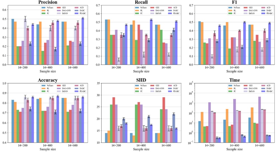
Figure 6. The performance of 6 metrics for 9 algorithms on 3 synthetic datasets. The horizontal axis represents 3 datasets of different sample sizes synthesised after selecting the first 200, 400 and 600 samples from 14 sub-datasets in turn, and the vertical axis represents the value of the evaluation metrics.
As demonstrated by Figure 6, as sample sizes scale up, PC, GES, and DAG-GNN uniformly display poor behavior across the six designated evaluation indices. This persistent performance bottleneck suggests that PC and GES get trapped in local optima due to their reliance on greedy search heuristics, whereas DAG-GNN enforces a strict structural acyclicity constraint that significantly degrades in accuracy when confronting systems with underlying cyclic features. Furthermore, owing to its reliance on a deep generative framework, DAG-GNN consistently demands the longest execution times. Both DiffAN and DABC exhibit high Precision scores but fall short in terms of Recall and F1 metrics; this disparity implies that both frameworks generate graph structures containing a high density of superfluous arcs. Conversely, ACD yields lower Precision, Recall, and F1 configurations but registers competitive profiles for SHD and Accuracy, a characteristic likely stemming from an under-parameterized network graph that contains too few total edges.
As the sample volume increases, the Precision and SHD trajectories of PDABC demonstrate continuous refinement, while its Recall, Accuracy, and F1 indices preserve their dominant positions, outperforming all baseline alternatives on the 14 × 600 matrix. While NoTears and RL occasionally achieve minor advantages over PDABC in isolated parameters, both models incur high computational overheads due to their respective deep generative and reinforcement learning architectures. In contrast, PDABC minimizes execution latency across all datasets, establishing a clear speed advantage that becomes increasingly pronounced as sample scales expand. A holistic review indicates that PDABC exhibits a more definitive performance profile than the other 8 comparative frameworks.
To objectively evaluate the global optimization capabilities of these methods, the 14 distinct sub-datasets are integrated into a single master matrix encompassing a total sample population of 11,672. Each algorithm is executed 10 times on this master matrix, with the resulting arithmetic means compiled in Table 5; the specific causal protein signaling topologies mapped by each framework are visualized in Figure 7.
Table 5. Comparisons of 9 algorithms on the total dataset with sample size of 11,672.
Algorithms | Time(s) | SHD | Accuracy | F1 | Recall | Precision |
No Tears | 35.30 | 15 | 0.84 | 0.45 | 0.47 | 0.44 |
RL | 797.01 | 15 | 0.84 | 0.45 | 0.47 | 0.44 |
PC | 10.56 | 25 | 0.72 | 0.32 | 0.47 | 0.24 |
GES | 11.60 | 30 | 0.69 | 0.27 | 0.41 | 0.20 |
DAG-GNN | 1582.00 | 24 | 0.67 | 0.27 | 0.29 | 0.25 |
DiffAN | 247.12 ± 2.54 | 16.15 ± 1.24 | 0.81 ± 0.07 | 0.32 ± 0.14 | 0.25 ± 0.26 | 0.43 ± 0.09 |
ACD | 293.16 ± 2.17 | 15.95 ± 0.67 | 0.86 ± 0.02 | 0.41 ± 0.02 | 0.35 ± 0.03 | 0.50 ± 0.02 |
DABC | 1.05 ± 0.03 | 12.30 ± 0.68 | 0.75 ± 0.01 | 0.38 ± 0.02 | 0.53 ± 0.02 | 0.29 ± 0.01 |
PDABC | 0.55 ± 0.01 | 15.90 ± 0.56 | 0.87 ± 0.01 | 0.53 ± 0.01 | 0.53 ± 0.01 | 0.53 ± 0.01 |
Note: The bold values indicate that the algorithm achieved the best results.
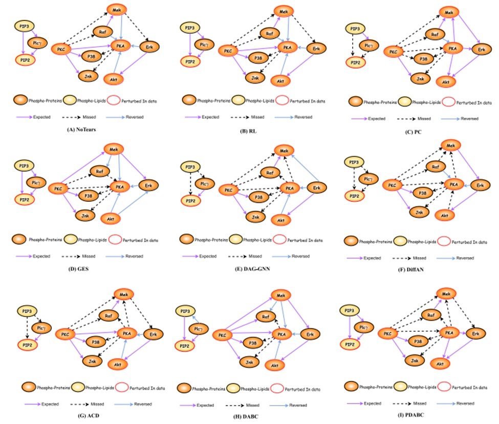
Figure 7. The causal protein signalling network learnt by 9 algorithms on single-cell data. Each graph contains three types of connected edges, indicating that the algorithm learns correct edges, missing edges, and reversed edges compared to the ground-truth network.
An integrated analysis of Figure 7 and Table 5 reveals that DiffAN and DAG-GNN correctly identify only 4 and 5 edges, respectively, while requiring considerable runtime allocations of 396 and 247.12 s. The performance profiles of these two models across most criteria fall substantially below the other comparison methods; this deficit is hypothesized to arise from the rigid directed acyclic graph (DAG) constraints embedded within their algorithms, which provoke a major drop in accuracy when resolving underlying cyclic topologies. The PC and GES frameworks each correctly resolve 7 valid edges, yet their Precision and Accuracy metrics are depressed by a high volume of false-positive redundant edges. NoTears and RL both successfully map 8 correct edges, but their operational architectures exhibit prolonged execution runtimes due to their deep learning and reinforcement learning sub-systems. The ACD approach maps 6 valid connections, yielding intermediate values across most evaluation indices without establishing clear architectural advantages.
Notably, both PDABC and DABC correctly resolve 9 out of 17 true edges, with both frameworks achieving a Recall score of 0.53. However, while DABC records an SHD value of 12.3—the lowest score among the compared methods—its Precision and F1 scores are restricted to 0.29 and 0.38, respectively. These values are significantly inferior to the 0.53 Precision and F1 scores generated by PDABC, confirming that the graphs produced by DABC are compromised by a high number of redundant edges. Furthermore, PDABC delivers an Accuracy score of 0.87, which is substantially higher than the 0.75 recorded by DABC. In terms of latency, DABC requires 1.05s of execution time, whereas PDABC requires only 0.55s, representing a near two-fold acceleration in processing throughput. Consequently, the global performance profile of PDABC is superior to that of DABC, validating that our proposed information fusion mechanism and parallelized search layout provide major functional advantages. In summary, the PDABC framework can successfully deduce causal protein signaling pathways with high stability and efficiency.
In this study, we presented a parallel discrete artificial bee colony (PDABC) optimization algorithm engineered to reconstruct causal protein signaling pathways directly from single-cell expression profiles. Empirical validation across both simulated models and real-world FACS single-cell matrices demonstrates that PDABC achieves higher performance and execution efficiency than contemporary state-of-the-art structure learning frameworks. The proposed framework successfully reverse-engineered and rapidly mapped the core topology of a causal pathway regulating human T-cell transduction, a key area of study within intracellular signaling networks. This network architecture was synthesized autonomously without relying on prior knowledge regarding pathway links. Deploying the PDABC framework across diverse cellular contexts featuring varying biomolecular targets, distinct cell lines, specific pathologies, and targeted experimental perturbations (including pharmaceutical agents, dominant-negative screens, and siRNA) can significantly accelerate the discovery of signaling mechanics. This approach offers particular value for decoding non-linear cross-talk across interconnected pathways, yielding insights into complex cellular dynamics and signaling interactions.
Although the present findings were derived from the quantification of 11 distinct phosphorylated molecules per cell, the steady evolution of analytical instrumentation and the capacity to track intra-cellular signaling cascades with high fidelity via advanced flow cytometry offer expanded horizons for identifying novel pathway topographies.
In certain contexts, the fundamental structural assumption of acyclicity required by standard Bayesian Networks may limit the capacity of PDABC to map causal protein pathways accurately, due to the high density of feedback loops within biological signaling cascades. However, when applied to time-series datasets, Dynamic Bayesian Networks (DBNs) possess the inherent capacity to model these recurrent feedback topologies. Consequently, migrating toward dynamic BN structures to reconstruct causal protein pathways represents a promising avenue for future research. A dynamic BN layout would allow the extraction of chronological data from time-ordered single-cell configurations, enabling the discovery of evolving causal network graphs. Concretely, the signaling network state at each discrete chronological unit can be treated as an individual Bayesian structural configuration; the global network can then be resolved from single-cell data by tracking modifications across consecutive states to quantify the dependencies among protein nodes and chart their temporal updates. Additionally, we plan to embed domain-specific prior knowledge, such as biological constraints governing protein interactions, directly into the model. Incorporating such insights can guide the choice of discretisation thresholds, mitigating information loss during data preprocessing and allowing the learned networks to mirror true biological causality with greater fidelity.
None
None
This work was partly supported by the National Natural Science Foundation of China Research Program (62106009, 62276010), in part by the R&D Program of Beijing Municipal Education Commission (KM202210005030, KZ202210005009).
None
Open Access The author(s) retain copyright. This article is licensed under the Creative Commons Attribution-NonCommercial-ShareAlike 4.0 International License. It may be shared and adapted for non-commercial purposes with appropriate attribution, an indication of changes, and distribution of adaptations under the same license. Third-party material may be subject to separate terms identified in its credit line. View the license at https://creativecommons.org/licenses/by-nc-sa/4.0/.
 Transparent Intelligence Publishing