Identifying vehicles within parking zones yields valuable insights into the spatial and temporal distribution of parking spot utilization. Because parking monitoring is conventionally conducted through manual observation, its temporal granularity remains restricted by substantial personnel expenditures. This study leverages simulated datasets alongside transfer learning to construct a dependable, real-world model tasked with detecting and categorizing vehicles via single-beam LiDAR within a roadside parking context. This work introduces a synthetically augmented transfer learning methodology designed for LiDAR-centric vehicle detection, alongside the deployment framework for synthetic LiDAR datasets. A synthetically augmented transfer learning technique was implemented to expand the constrained real-world dataset and facilitate the formulation of data management workflows. Furthermore, incorporating this synthetically augmented transfer learning methodology enhances both the resilience and the overall precision of the network. Empirical tests demonstrate that this approach enables the rapid deployment of models tailored for vehicle detection using a LiDAR sensor.
In modern urban environments, municipal authorities and urban planners face a primary obstacle in mitigating the ecological degradation caused by traffic jams. Within the UK specifically, the DEFRA (UK Government Department for Environment Food & Rural Affairs, London, UK) clean air strategy incorporates a £3 billion initiative targeted at elevating air quality standards and curtailing hazardous vehicular emissions. Furthermore, approximately 30% of metropolitan traffic congestion is generated by motorists seeking available parking spots, with UK drivers squandering an annual average of nearly two full days (44 h) looping urban roadways to locate vacant spaces—a figure that escalates to nearly three full days (67 h) for those in London. Additionally, roughly 33% of parking infrastructure remains underused on any given day [1], establishing parking regulation as a fundamental pillar of viable traffic management, particularly within densely populated metropolitan centers.
The domain of parking management has undergone relatively minimal academic investigation upon which future smart city frameworks can be established [2]. This deficit stems largely from the reality that numerous municipalities lack foundational inventories regarding their parking assets [3], especially concerning curb-space parking, due to the intensive labor requirements associated with acquiring such information via classic, manual parking assessments [2]. Granular datasets characterizing parking space utilization across specific temporal and spatial zones would offer critical perspectives, highlighting the parking demands, behaviors, and tendencies of drivers [4, 5]. Nonetheless, on-street parking resists straightforward evaluation due to the vast and scattered nature of the target temporal and spatial spans. Conventional approaches for executing curb-space parking assessments involve personnel walking or driving through designated zones to manually count stationary automobiles, which typically yields only coarse metrics such as aggregate occupancy percentages [2]. Consequently, data derived from these practices are utilized to understand broad regional parking patterns rather than real-time spot availability, which could otherwise guide motorists planning trips into urban centers [2]. A technique capable of autonomously determining parking space availability in metropolitan sectors would alleviate gridlock and environmental pollution in downtown cores, while simultaneously enhancing driver convenience and boosting regional economic productivity. In practice, automated traffic surveillance relies on a variety of sensor architectures for vehicular applications, including inductive loops, subterranean road sensors, radar units, and Bluetooth detectors [6]. Inductive loop detectors provide dependable and economical performance for identifying automobiles, operating traffic signals, and regulating vehicle streams, yet they demand ongoing upkeep and are susceptible to environmental degradation [7]. Subterranean road sensors are resilient and gather precise metrics regarding traffic volume, spot occupancy, and vehicular velocity, but their installation and maintenance can be financially demanding [8]. Radar units deliver precise tracking and capture a diverse array of vehicle classes and dimensions, though they can suffer from electromagnetic disruptions [9]. Bluetooth detectors represent an inexpensive and easily deployable option, but their utility is restricted by the baseline prevalence of active Bluetooth-enabled devices [10]. These conventional sensing modalities generally yield aggregate traffic volume counts at fixed positions rather than high-resolution, micro-level traffic metrics such as individual velocity, precise positioning, heading, and specific timestamps [11].
More recently, advanced high-fidelity sensing platforms, computer vision frameworks, and LiDAR instruments have been deployed across numerous scenarios to gather high-resolution traffic intelligence for identifying automobiles, pedestrians, pavement edges, roadside infrastructure, and driving lanes. Vision-based systems and LiDAR hardware offer marked enhancements in monitoring distance and precision relative to legacy traffic surveillance instruments [12-14]. Nevertheless, optical camera configurations exhibit suboptimal performance when encountering intricate settings with highly variable lighting parameters [11], and concerns regarding public privacy can restrict their geographical installation options. Current strides in the high-volume, low-cost fabrication of LiDAR hardware enable the cost-efficient installation of units along roadsides to supply high-resolution, micro-level traffic datasets. These sensor systems rely heavily on subsequent post-processing routines that utilize diverse analytical strategies to extract actionable patterns from the gathered data. These techniques span from elementary rule-based feature isolation to cutting-edge, data-driven methodologies. Even so, multiple roadblocks persist when deploying economical LiDAR configurations for the real-time identification and tracking of vehicles. A primary obstacle for data-driven architectures is the scarcity of high-quality, annotated reference datasets. This issue is particularly acute when engineering solutions around emerging hardware since the absence of historical data precludes the initial training of a data-driven model. The academic community is addressing this barrier across diverse fields by capitalizing on virtual data generation and transfer learning mechanisms [15-17]. Transfer learning represents a training methodology through which a machine learning architecture optimized for a specific source domain can be adapted and repurposed to construct a new model within a separate target domain, or to execute a distinct yet correlated objective. Within transfer learning frameworks, a frequent dual-stage strategy to mitigate data deficiencies entails pre-training an architecture on massive quantities of synthetically produced data and subsequently adapting this network using a restricted corpus of empirical, real-world data [18]. While this workflow has been broadly embraced within computer vision applications [19], sparse investigation has targeted its utility in bolstering the stability and precision of vehicle detection models engineered for low-cost, mass-produced LiDAR hardware. The existing literature defines multiple classifications of transfer learning, such as homogeneous, heterogeneous, inductive, and transductive variants [20, 21], alongside distinct operational methodologies, specifically feature-based and model-based transfer learning [20]. This investigation adopts an inductive form of transfer learning, utilizing a feature-based methodology to execute the knowledge transfer.
This study fills the identified research deficit by introducing a novel strategy that employs synthetic data augmentation to formulate a resilient, data-driven architecture for vehicle detection optimized for an innovative signal acquisition methodology, namely economical single-beam LiDAR hardware, designed for field implementation. Following comprehensive validation procedures, the evidence indicates that the introduced workflow improves the precision of the vehicle forecasting objective relative to standard transfer learning executed without synthetic data augmentation.
This section reviews the academic environment regarding multi-model vehicle and object categorization within traffic management scenarios. LiDAR and video systems represent the two most prevalent sensing options utilized to identify vehicle presence, with each technology offering specific pros and cons. In the domain of vehicle tracking, camera-derived data is highly intuitive for human interpretation and simplifies the data labeling workflow; consequently, it has served as the foundation for numerous methodologies [11, 22]. These strategies process image data acquired by standard cameras, where individual pixels represent grayscale or color intensity, requiring objects to be identified and isolated (establishing boundaries) before their spatial coordinates can be determined. Furthermore, this process can become intensely problematic under dim lighting environments, such as night conditions, where the colors and edges of objects become increasingly difficult to distinguish.
Deploying instruments based on LiDAR technology offers a viable approach to circumventing these constraints. Processing LiDAR data can be more computationally streamlined and delivers efficient monitoring across both close and extended ranges compared to standard camera captures [2, 23]. LiDAR gathers high-fidelity point clouds—which constitute datasets detailing the precise distance from the emitter to the surfaces within a scene—meaning that the spatial position and scale of target objects are inherently embedded within the raw measurements. Moreover, because LiDAR evaluates the reflected signal of light emitted directly by the instrument, ambient atmospheric and lighting conditions exert negligible influence on the collected data. Concurrently, recent innovations in the high-volume, low-cost manufacturing of LiDAR hardware facilitate the acquisition of high-resolution micro-traffic metrics.
Two distinct paradigms are conventionally utilized for identifying and classifying vehicles using roadside-mounted LiDAR data: feature-based frameworks and data-driven frameworks.
Feature-based frameworks employ handcrafted feature isolation techniques—such as extracting vehicle height, width, length, and central dip profiles—from the LiDAR signal to categorize automobiles. Under this paradigm, LiDAR streams can be exploited for vehicle tracking through several mechanisms; for instance, the recorded LiDAR distance drops when an automobile intercepts the laser beam, allowing the corresponding vehicle height to be determined via elementary geometric calculations [24]. In another study, Ref. [25] isolated dependable features to facilitate supervised vehicle categorization using LiDAR profile streams as inputs. Similarly, Ref. [26] engineered an analytical routine to extract high-resolution vehicular trajectories from roadside LiDAR telemetry, applying these paths to evaluate traffic efficiency. Additionally, Ref. [27] designed a laser-centric vehicle classification framework relying on diverse criteria, including geometric layouts, occlusion modeling, hardware specifications, and tracking telemetry. Frequently, the features extracted via these handcrafted methodologies are routed into various classical classification algorithms, including decision trees, support vector machines, and principal component analysis [28]. Although these methodologies are straightforward and efficient, they exhibit vulnerability to noise and complex environments; for example, they fail to adequately manage severe occlusions, as deduced from [27, 28].
Data-driven frameworks employ diverse neural network topologies to execute classification tasks on the 3D point clouds produced by LiDAR hardware [29]. Recently, Convolutional Neural Networks (CNNs) have attained remarkable benchmarks in object identification objectives across both camera and LiDAR domains. Multiple investigations [30-32] utilize imagery recorded by optical cameras and implement unified, end-to-end fully convolutional network architectures that simultaneously estimate object probability scores and spatial localization (bounding coordinates). Furthermore, the scope of object tracking and localization has expanded to embrace 3D LiDAR arrays within automated piloting frameworks [33]. Chen et al. [34] blended LiDAR point cloud features with localized image characteristics through a region-centric fusion network to resolve the 3D localization objective and 3D object tracking, surpassing alternative LiDAR-only methods in 2D tracking when evaluated against the open-source KITTI benchmark repository [35].
Two primary difficulties emerge when applying retrofitted LiDAR scanners to existing street infrastructure in practical deployment scenarios. First, these scanners are integrated with and managed by resource-constrained IoT hardware, which exhibits limited processing capacity and introduces data latency due to wireless transmission links. Second, the physical mounting location on lampposts causes the collected telemetry to suffer from frequent vehicular occlusions, as depicted in Figure 1. Object tracking frameworks are routinely utilized to identify vehicles within static images and video feeds. Multiple prominent object tracking algorithms exist, including YOLO (You Only Look Once) [36], SSD (Single Shot MultiBox Detector), and Faster R-CNN (Region-based Convolutional Neural Network) [37]. These models are built upon deep learning structures—specifically Convolutional Neural Networks (CNNs)—which have demonstrated high efficacy for image interpretation objectives and are widely recognized for their flexibility and open-source availability. Each architecture possesses specific advantages and deficiencies. YOLO is distinguished by its operational velocity and real-time responsiveness, making it highly suitable for environments like self-driving systems. SSD achieves an effective trade-off between processing speed and tracking precision, rendering it another prevalent selection for vehicle tracking applications [38]. Conversely, Faster R-CNN is noted for its high accuracy and is frequently deployed for object monitoring tasks due to its competence in identifying hidden targets [39]. It utilizes a region proposal network to isolate candidate object zones, enabling it to detect vehicles even when they are partially blocked or obscured by other entities in the environment [40], a capability that is highly advantageous for our vehicle parking application. Investigation [38] established that the Faster R-CNN architecture maintains a well-balanced recall-to-precision ratio; conversely, YOLOv3 demonstrates a higher recall relative to its precision, indicating that YOLOv3 generates a greater frequency of false classifications. Consequently, Faster R-CNN was selected exclusively to execute all operations within the introduced workflow.
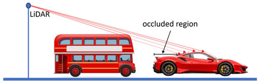
Figure 1. Occluded region of the vehicle. The car is partially occluded by the bus parked behind it.
One of the most persistent bottlenecks encountered by data-driven frameworks—such as CNN, RCNN, and Faster R-CNN—within field deployments is the shortage of extensive, human-annotated datasets [41]. In scenarios lacking sufficient real-world telemetry, high-fidelity synthetic datasets have been successfully implemented across numerous fields [42-44]. For instance, Wang et al. [41] produced synthetic imagery spanning both photorealistic and non-photorealistic styles, subsequently employing a transfer learning strategy for vehicle tracking via a Faster R-CNN framework. Transfer learning enhances the training phase of a novel objective (the target domain) by migrating insights acquired from a correlated, previously resolved objective (the source domain) [45]. Specifically, transfer learning optimizes model capability by initializing training with the foundational weights derived from a baseline model [45] and then refining these parameters using a constrained data sample from the target objective. It follows that these foundational networks must be thoroughly optimized and validated to ensure superior terminal capabilities. Additionally, transfer learning removes the rigid constraint that training and evaluation datasets must share identical statistical distributions [46]. This flexibility has benefited numerous disciplines plagued by insufficient training data, including signal denoising, botanical sciences, seismic fault characterization, structural degradation tracking, and hazard forecasting [47, 48]. Nonetheless, the two underlying datasets must share contextual commonalities; transfer learning cannot function if no logical correlation connects the domains.
Within transfer learning paradigms, two primary implementation options are typically pursued: feature extraction and fine-tuning [48]. In the feature extraction workflow, all internal parameters of the source domain neural network are locked (or frozen), with the exception of the terminal fully connected layer (frequently denoted as the softmax layer). The multi-dimensional array from the terminal output of these locked layers is isolated and flattened into a feature vector, which subsequently serves as the input to train an independent classifier, such as a multilayer perceptron or a Support Vector Machine (SVM), to resolve the target objective [49]. In the fine-tuning workflow, a straightforward technique involves optimizing all parameters throughout the deep architecture using the target domain training samples. However, optimizing the entire network architecture can precipitate overfitting if the target sample pool is restricted. Alternatively, the parameters governing the initial layers can remain frozen at their pre-trained values, while only the final layers of the deep network are fine-tuned. Depending on the scale of the dataset, the structural complexity of the task, and the targeted precision benchmarks, these two options can be strategically selected for different use cases [48].
This document introduces a methodology for the occlusion-resilient localization, detection, and categorization of vehicles utilizing an inexpensive, single-beam LiDAR sensor. A Faster R-CNN architecture is trained on simulated datasets using transfer learning mechanisms. While a small number of investigations have explored synthetic-to-real transfer learning across different domains and use cases [47, 48], this research represents the initial study to implement synthetic-to-real transfer learning utilizing roadside LiDAR sensor streams for vehicle tracking objectives. Furthermore, this workflow is validated on actual, field-collected LiDAR data for vehicle tracking. The primary innovations delivered by this study comprise:
A dedicated utility for generating synthetic LiDAR data.
A comprehensive performance evaluation of transfer learning executed with and without simulated datasets:
Transitioning from camera-derived real-world datasets directly to our specialized LiDAR data streams.
Transitioning from camera-derived real-world datasets, through an expansive synthetic data repository that models our real-world dataset precisely, to our specialized LiDAR data streams.
This comparative analysis reveals that, within our specific use case, Synthetically Augmented Transfer Learning drives a measurable increase in the precision of the categorization framework.
This investigation evaluates and enhances an object detection framework optimized through two distinct transfer learning baselines: first, utilizing an extensive image repository acquired via a different modality (namely, optical cameras) relative to our operational datasets (LiDAR); and second, incorporating an intermediate phase leveraging a substantial synthetic dataset that precisely models our empirical roadside LiDAR telemetry. The core research architecture of this study is outlined in Figures 2 and 3. Figure 2 illustrates the Classic Transfer Learning paradigm, where a pre-trained Faster R-CNN object detection architecture developed using the Common Objects in COntext (COCO) repository [50] serves as the baseline framework, from which knowledge is subsequently transferred to our empirical LiDAR stream. Figure 3 delineates the Synthetically Augmented Transfer Learning paradigm, wherein a large-scale, artificially generated dataset is integrated into the transfer learning pipeline prior to finalizing network adaptation with the empirical LiDAR telemetry.
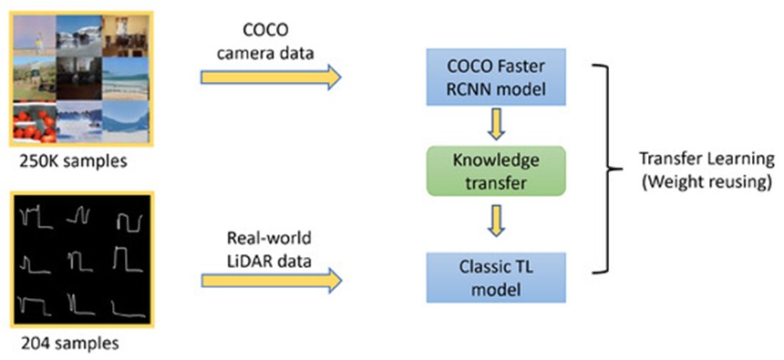
Figure 2. Classic Transfer Learning method: Classic TL model is transfer learned using real-world LiDAR data from the COCO Faster R-CNN model.
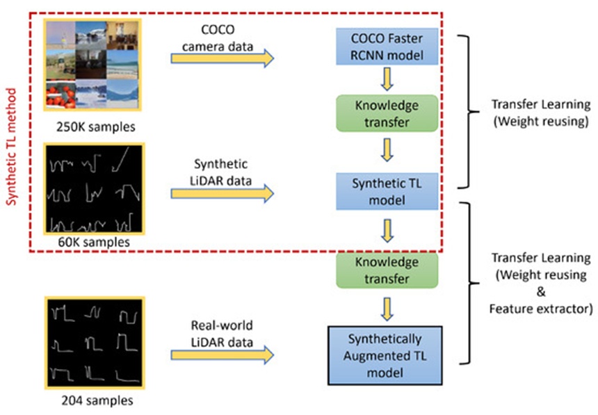
Figure 3. Synthetically Augmented Transfer Learning method: Synthetically augmented TL model is transfer learned using real-world LiDAR data from the Synthetic TL method, whereas the synthetic TL model is transfer learned using synthetic LiDAR data from the COCO Faster R-CNN model.
This section details the simulation framework designed to yield the virtual data streams on which the network is optimized to identify, locate, and categorize vehicles embedded within the LiDAR signal. The virtual environment is structured around two primary scene components: the roadside-mounted LiDAR configuration and the 3D vehicular assets. The vertical distance, p_h, between the target vehicle surface coordinate and the ground plane, as illustrated in Figure 4, is evaluated and used to construct the cross-sectional vehicular profile imagery.
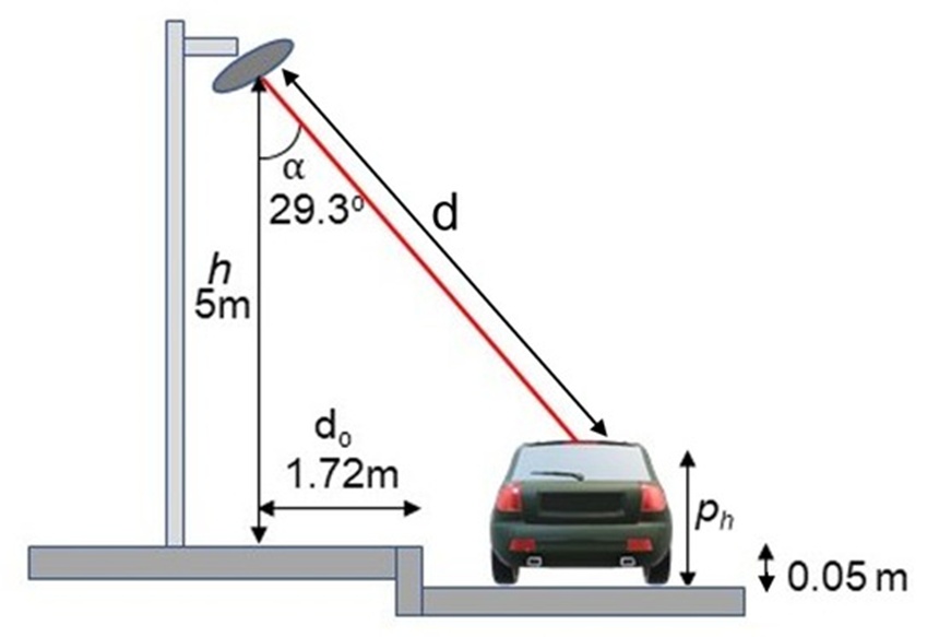
Figure 4. Illustration of our LiDAR system.
Within this simulated LiDAR configuration, the ground surface serves as the baseline reference plane for calculating distance measurements; note that the LiDAR unit itself functions as the zero-reference node within the real-world operational system. As depicted, the linear range d between the LiDAR emitter and the target surface coordinate, the height h dividing the LiDAR unit from the ground plane, the inclination angle 𝛼 between the emitted laser beam and the vertical axis, and the resultant elevation ph separating the surface intersection point from the ground are systematically derived. This computation is executed using the principles of ray-triangle intersection, given that each 3D vehicular asset is composed of an array of triangular facets provided by the ShapeNet repository [51].
Our simulation environment instantiates numerous distinct scene layouts to construct a diverse repository of LiDAR profiles meant to replicate empirical field conditions. This section reviews the selected implementation strategies along with the foundational mechanisms of the simulation system.
The 3D assets obtained from ShapeNet adhere to a standard structural format (.obj) that describes a shape as a triangular mesh topology, meaning that the outer boundary of the 3D entity is composed of numerous triangular polygons linked along their shared boundaries. These meshes are imported into our software pipeline, which leverages their triangular configuration to calculate highly accurate spatial positions for the LiDAR ray intersections. The ShapeNet 3D vehicular models are categorized into nine distinct classes: Car, 4 × 4, Van, Motorcycle, Bicycle, Bus, Truck, Double-Decker, and Minibus, which are displayed in Figure 5. This study delivers performance benchmarks based initially on seven categories and subsequently on five categories when aligned with empirical datasets; a collection exceeding 5,000 distinct models, each yielding an individual LiDAR signature, was utilized across our testing routines. Selecting diverse arrangements of these geometric shapes alongside other operational parameters, as outlined in Table 1, allows us to generate a massive, highly varied repository of LiDAR signatures.
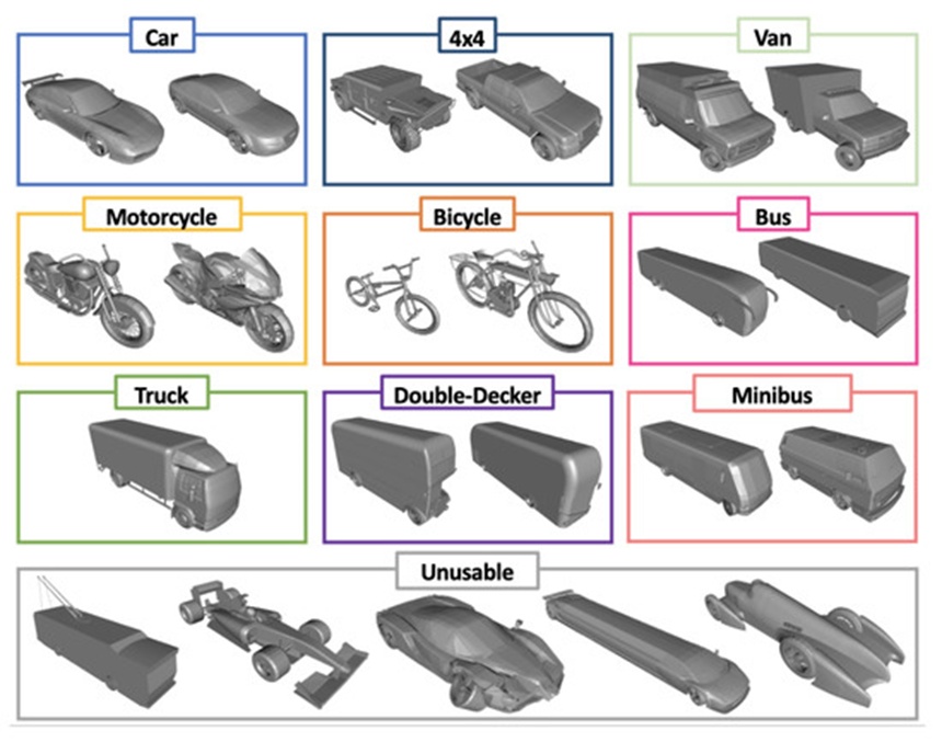
Figure 5. ShapeNet 3D Vehicles, split into nine classes: Car, 4 × 4, Van, Motorcycle, Bicycle, Bus, Truck, Double-Decker, and Minibus.
Table 1. Parameters and assumptions.
Parameter | Symbol | Description | Type | Value |
LiDAR Mounting Height | h | Vertical separation between the LiDAR sensor and the road surface | Fixed | 5 m |
LiDAR Lateral Offset | dₒ | Horizontal distance from the LiDAR location to the road curb | Fixed | 1.72 m |
LiDAR Orientation Angle | α | Tilt angle of the LiDAR used for roadway observation | Fixed | 29.3° |
LiDAR Angular Resolution | Lᵢ | Angular step traversed by the LiDAR between consecutive measurements | Fixed | 1° |
Observation Arc | Lₐ | Angular range defining the region of interest for data collection | Fixed | 120° |
Scan Frequency | Lₛf | Rate at which the LiDAR completes repeated scans | Fixed | 5.5 Hz |
Scan Duration | Lₛt | Time required for the LiDAR to complete a full angular sweep | Fixed | 0 s |
Detection Range | Lᵣ | Maximum distance from the sensor at which valid measurements are returned | Fixed | 12 m |
Vehicle Model | Vₜ | Vehicle instance selected from the ShapeNet dataset (SN) | Variable | ∈ SN |
Vehicle Scaling Factor | Vₛ | Three-dimensional scaling applied to the vehicle relative to the scene and other dataset vehicles | Fixed | — |
Vehicle Travel Direction | Vd | Direction of motion, represented as forward (F) or backward (B) | Variable | ∈ {F, B} |
Vehicle Heading Angle | θ | Orientation of the vehicle relative to the road curb | Variable | θ ~ U(−9, 9) |
Measurements per Revolution | Sᵣ | Number of individual LiDAR samples collected during one complete rotation | Derived | 720 |
Measurements per Second | Sₜ | Total number of LiDAR measurements acquired each second | Derived | 3960 |
Measurements within Observation Arc per Second | Sₛₜ | Number of LiDAR measurements per second that fall within the observation arc Lₐ | Derived | 1320 |
Number of Parked Vehicles | mᵥ | Total count of parked vehicles included in the scene | Fixed | 5 |
To simulate the physical properties of a LiDAR sensor, it is necessary to determine the geometric intersections between linear trajectories originating from our virtual LiDAR instrument and the rendered vehicular asset. A computational methodology known as ray casting is deployed to achieve this goal. Ray casting operates by defining a specific origin within 3D space along with a vector indicating the target propagation heading, subsequently tracking the virtual 3D environment to record any intersections with solid models. Each discrete angular increment of the LiDAR system's rotational sweep projects a single ray and classifies the resulting contact into one of three outcomes: a vehicular asset intersection, a roadway plane intersection, or a non-intersection event. These distinct trajectories are visualized in Figure 6. Ray casting not only allows us to determine if a given trajectory intersects an entity but also establishes the exact spatial coordinates of the contact zone and the absolute length of the ray path. A specialized rendering software package designated as VTK (Visualization Toolkit) was used to execute the ray casting operations and intersection calculations [52] for the construction of our synthetic database.
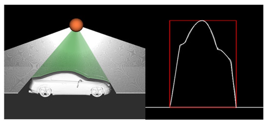
Figure 6. Rendering of the intersections between LiDAR rays and a vehicle’s surface, the left image shows how the LiDAR ray intersects the 3D vehicle model, and the right image shows the generated 2D profile image (scaled).
An array of ambient field variations alters the telemetry captured by physical LiDAR hardware. Our validation routines seek to emulate many of these external factors to enhance the realism of our simulated datasets. This section presents several developed strategies.
Vehicles do not consistently park directly underneath and parallel to the roadside LiDAR deployment; consequently, our simulation routines incorporate rotational adjustments to the vehicular assets. To achieve this data enhancement, the target model is rotated within 3D space around a designated coordinate line, the Y-axis. In this framework, the 3D coordinate system is aligned such that the Y-axis extends vertically upwards, the X-axis projects perpendicular to the roadway alignment, and the Z-axis runs parallel to the flow of traffic. It follows that executing the rotational calculation around the Y-axis is sufficient to alter the orientation of the vehicle in a realistic manner, assuming the model is originally positioned parallel to the Z-axis line. The Y-axis rotational transformation matrix defined in Eq. 1 is applied to every coordinate vertex comprising the 3D mesh to induce an angular shift of \theta^\circ, which is varied randomly for each vehicular model across different scenes to maximize the structural diversity of the training set. A sample rendering illustrating vehicular orientation adjustment is shown in Figure 7.
 (1)
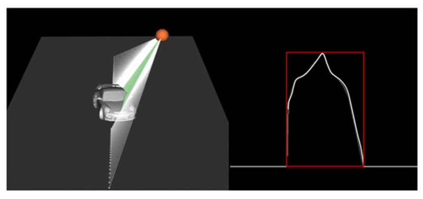
Figure 7. Rendering of a vehicle passing the LiDAR sensor at an angle, \theta, from our simulations.
Each vehicle is positioned within the scene (consistently, at minimum partially beneath the LiDAR) across a diverse spectrum of locations relative to the X-axis and Z-axis, incorporating adjustments to the vehicle orientation. Multi-vehicle Scenes are generated by employing a random assortment of vehicle profiles. Given that our installed real-world LiDAR sensors generally monitor parking areas, most scans are expected to feature multiple stationary vehicles mv. To ensure the trained model performs robustly under conditions of occlusion, as illustrated in Figure 1, it is essential to apply transfer learning to scenarios with multiple vehicles parked at various intervals beneath the LiDAR sensor (a representative instance is displayed in Figure 8). In contrast to real-world datasets, because the specific vehicle types utilized in each scene are pre-identified, the corresponding labels can be generated with ease.
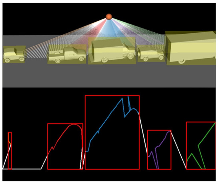
Figure 8. Rendering of five vehicles parked along with the resulting LiDAR image.
The preceding sections have emphasized the primary variables involved in generating the vehicle profile scenes. This section details a comprehensive inventory of the parameters accounted for during the computation of synthetic LiDAR data, which are outlined in Table 1.
As indicated in the third column, these parameters are classified into two main categories: fixed and variable parameters; additionally, there are derived parameters, which are computed from other primary variables. These parameters are selected to accurately reflect our real-world environment; a visual representation of the LiDAR setup along with its associated parameters is provided in Figure 4.
This section details the model training phase employing the synthetic TL approach, which is framed by the dashed red box in Figure 3, using Faster RCNN as the underlying framework. The synthetic dataset comprises a training set of 60,000 instances, a validation set of 14,425 instances, and a evaluation dataset of 43,272 instances, with each set containing observations spanning seven separate classes. Initially, a pre-trained Faster RCNN [50] architecture built on ResNet and trained on the COCO dataset was selected as the foundational model. The Faster RCNN framework is divided into three distinct components: convolutional layers, where filters are optimized to extract relevant features from the input imagery; a Region Proposal Network (RPN), which processes the final CNN feature map to estimate potential object proposals; and a fully connected layer, which determines the final object classifications and bounding boxes. This architecture is optimized utilizing stochastic gradient descent.
Subsequently, the model is adjusted using the weight-reusing transfer learning strategy; specifically, the original Faster RCNN model is taken, its terminal layer is discarded, our custom classification layer is integrated, and the newly configured model is trained. All network weights are updated during training on the synthetic dataset over 25,000 total steps, which includes 2,000 warm-up steps. A few basic preliminary tests adjusting the total steps and warm-up intervals were performed; however, they yielded no substantial impact on the learning trajectory, leading to the adoption of the parameter configurations recommended in [53]. Ultimately, the transfer-learned object detection model is evaluated against the synthetic test dataset. This workflow is consistently applied across all experimental tasks in this research.
Figure 9 displays the confusion matrix derived from the synthetic test dataset across the 43,272 total samples. The diagonal components indicate the percentage of accurately predicted classes, whereas the off-diagonal components represent the error distribution percentages for each respective category. The overall classification accuracy reaches 88.36%; as illustrated, the Bus and Double-Decker categories present the greatest classification challenges, yielding accuracies of 68% and 62%, respectively. Furthermore, the algorithm demonstrates strong capability in localized vehicle detection within the scene, as quantified by the mean and variance of the Intersection over Union (IoU) metric defined in Eq. 2; these values are recorded at 0.88 and 0.23, respectively.
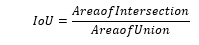 (2)
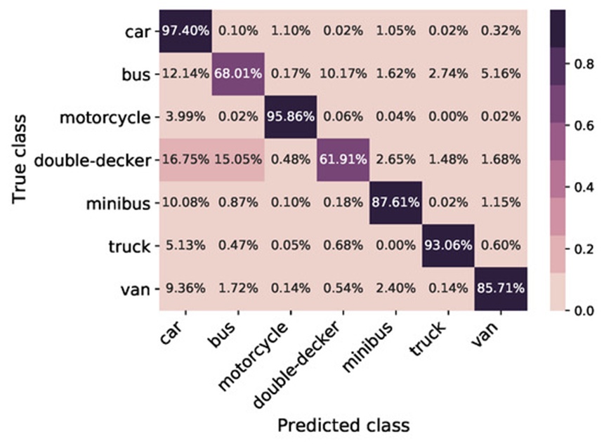
Figure 9. Confusion matrix of test data set for 43,272 total samples; classification accuracy—88.36%.
Figure 10 presents the Receiver Operating Characteristic (ROC) curve evaluated on the test dataset across all categories. The X-axis represents the false positive rate, while the Y-axis tracks the true positive rate. The plot demonstrates that all categories are predicted accurately, yielding an Area Under the Curve (AUC) ranging between 0.97 and 1.
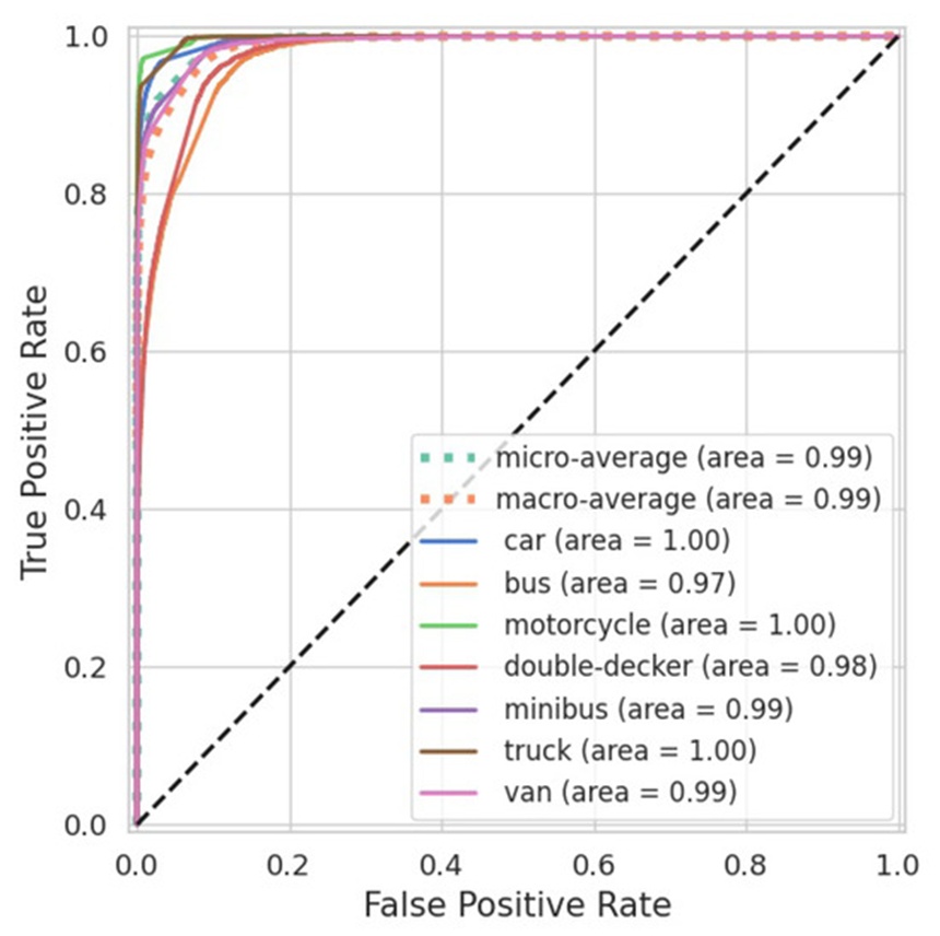
Figure 10. ROC curve of the test data set for 43,272 samples.
Following the validation of a functional model utilizing synthetic data, this section details the deployment of the LiDAR hardware, the collection of range data from the sensor, and the subsequent data pre-processing steps required to evaluate the real-world performance of the synthetically trained Faster RCNN model.
The hardware deployed is the Slamtec RPLIDAR S1, which utilizes time-of-flight (ToF) ranging technology to ensure a measurement accuracy of +/-5\text{ cm} across its entire operational range. It maintains a stable and precise ranging resolution even over extended distances. Furthermore, it successfully mitigates significant daylight interference, delivering reliable ranging and high-resolution mapping capabilities in outdoor environments. The sensor is compact, user-friendly, portable, and sufficiently lightweight to accommodate various application demands. The RPLIDAR S1 rotates clockwise to execute a 360-degree omnidirectional laser range scan of its environment (Figure 11). Additionally, this system integrates wireless power, optical communications, and non-contact energy and signal transmission technologies to replace traditional slip rings or other physical links prone to mechanical wear and shortened operational lifespans [54].
This specific device was chosen because it offers a favorable balance of affordability, compact dimensions, extensive range, and a high scanning frequency. While a 3D LiDAR sensor would offer distinct advantages, the financial cost of such equipment is orders of magnitude greater, and processing their outputs requires significantly higher computational resources due to the massive volume of data generated. Owing to COVID-related restrictions throughout the majority of this funded research, the installation of the LiDAR for real-world data collection was confined to a single geographic location.
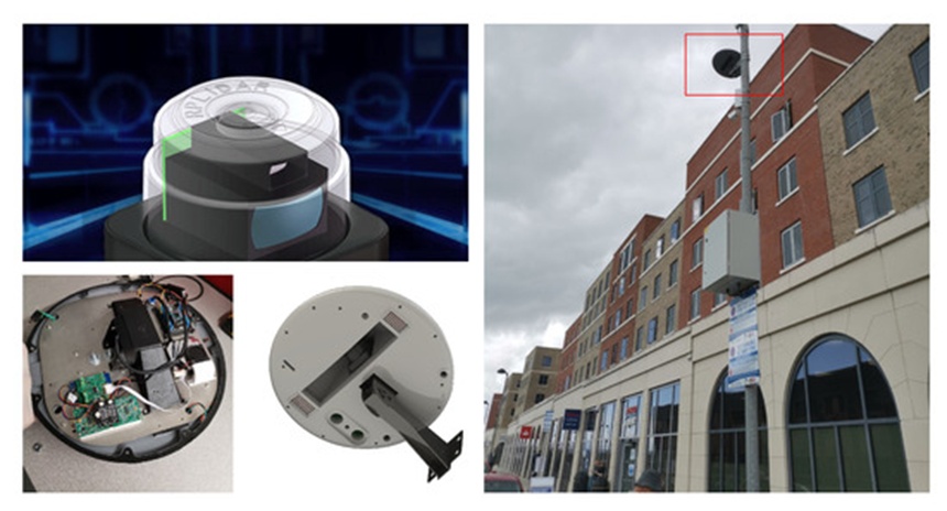
Figure 11. LiDAR hardware installation.
The LiDAR sensor scans the designated environment and streams the collected information to cloud storage in real time. For every second of operation, the LiDAR system samples ten frames per second (ten sequences of 360 measurements, captured at 1∘ intervals per sample) and logs these data points in polar coordinates within a MySQL database. These entries are retrieved via SQL queries for specified time windows and contain: the scan angle 𝛽 measured in degrees and the distance (d) measured in millimeters. In this context, 𝛽 denotes a specific angle within the defined Arc of Interest La at that precise moment. Although the LiDAR records a full 360-degree field of view, the target focus is restricted to the segment where the laser intersects the roadway, which spans 120 degrees, La. An illustrative example comparing a polar plot to a polar-to-Cartesian transformation is provided in Figure 12, showcasing the zone where the LiDAR monitors the street. Within the polar representation, the polar coordinates (d, 𝛽) map out the captured vehicle profiles alongside the road surface. These polar points are converted into Cartesian coordinates (𝑥=𝑑cos(𝛽),𝑦=𝑑sin(𝛽)) to facilitate the analysis of vehicle profiles. The data visualized in Figure 12 reflect raw sensor outputs and include noise and measurement artifacts that must be filtered out to enable successful object detection.
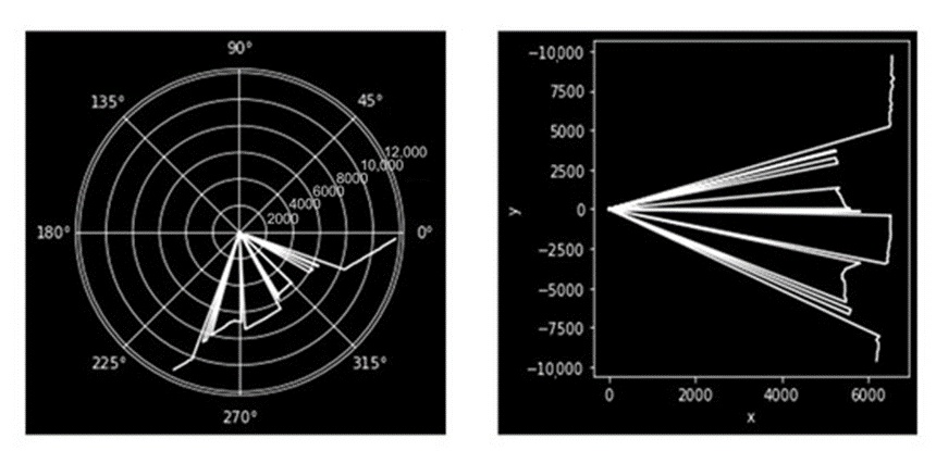
Figure 12. Polar plot (left) and polar to Cartesian Plot (right) of the LiDAR data.
Not all real-world LiDAR measurements yield pristine vehicle profiles. To extract a usable profile from the Cartesian plot, several noise reduction and filtering operations had to be implemented, as specified below:
Eliminate LiDAR points that register excessively close to the sensor. Under certain environmental conditions, the device can generate very small or zero distance readings instead of valid measurements.
Constrain the data range between 3000 and 7000 mm to isolate only the relevant vehicle profiles within the Cartesian plot shown in Figure 12.
Suppress the frame when no vehicles are stationary on the roadway by restricting the x values between 6000 and 7000 in the Cartesian plot of Figure 12.
Discard any LiDAR frames that periodically generate deficient profiles, which occurs when a vehicle profile is not adequately captured; for example, when the LiDAR intersects a rapidly moving vehicle, it frequently registers merely a vertical line that conveys no useful structural data.
Normalize the image scale by limiting the dimensions of the x and y-axes to align with the proportions of the synthetic training data.
The vehicle profiles displayed in Figure 13 (left), paired with the corresponding real-time photograph of parked vehicles (right), have been prepared using the data processing workflow described above.
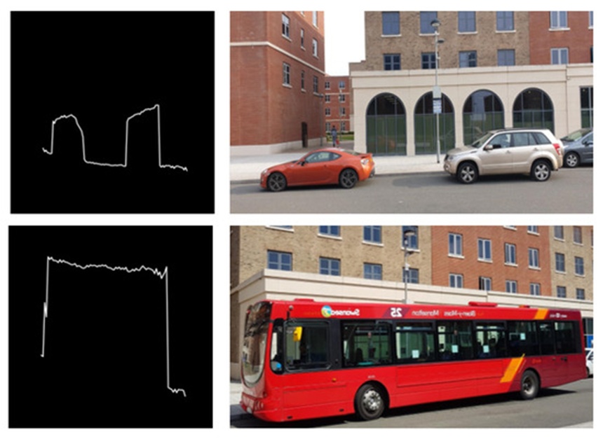
Figure 13. Samples of processed LiDAR image (left) and vehicle parked in real time (right).
To evaluate the real-world performance of the system upon deployment, it is necessary to establish a baseline of ground truth labeled data. This subsection details the development of a semi-automated labeling pipeline for the LiDAR data, utilizing video feeds recorded by cameras attached to a lamppost at the deployment site.
The camera infrastructure consisted of two IP cameras (RLC—410W) fixed to the same lamppost supporting the LiDAR sensor. Each camera features an 80-degree field of view, thereby collectively encompassing the 120-degree operational range of the LiDAR. These cameras feature integrated motion detection sensors that initiate video recording, thereby filtering out irrelevant footage. The cameras recorded continuously around the clock, and the accumulated data files were transferred and stored via file transfer protocol (FTP).
An image-based object detection framework was deployed to generate labels for the dataset, leveraging the fact that this domain is highly developed and offers numerous pre-trained models capable of executing this task efficiently. In particular, the YOLO (You Only Look Once [55]) framework and its subsequent iterations (YOLO V1, V2, V3, V4, and V5) have consistently demonstrated performance that exceeds alternative state-of-the-art object detection methodologies. The YOLO_V5 model was selected for this study due to its 53.7% mAP (mean Average Precision) on the COCO dataset [56], outperforming YOLO_V4 which achieves a 43.5% mAP on COCO [57], alongside its straightforward deployment and execution speed. Despite these advantages during our evaluations, the model occasionally misidentified certain vehicles. It is hypothesized that the primary factor driving these misclassifications was the camera mounting angle coupled with the high density of objects within the frame. Figure 14 highlights two distinct errors; in the left image, on the far left boundary, a vehicle is erroneously classified as an incorrect object class (indicated by the green bounding box); in the center, a vehicle is identified accurately (orange bounding box), whereas on the right, a vehicle fails to be detected entirely. In the right image, the objects are correctly identified as cars; however, on the leftmost edge of this frame, a partially visible vehicle is omitted from classification.
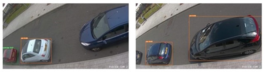
Figure 14. Object detected by YOLO_V5 model for images captured in different angles.
By applying a confidence threshold and filtering exclusively for the target categories (Car, Bus, Motorcycle, Minibus, and Van), an initial baseline reference was constructed, as presented in Table 2, documenting the class, bounding box coordinates, prediction confidence score, timestamp, and a Boolean daytime indicator. This ground truth label is subsequently associated with the LiDAR dataset by aligning identical timestamps, followed by a final manual validation stage to guarantee the precision of the generated labels. We observed a decrease in tracking accuracy for the camera-derived data during nighttime hours (demarcated as the period after sunset and before sunrise), exhibiting a 43% drop in accuracy relative to daytime conditions. Following manual correction, a robust dataset consisting of 303 annotated LiDAR images was produced, from which 413 distinct LiDAR profiles were extracted. The volume of LiDAR samples available for evaluation was constrained by COVID-related public movement restrictions enacted during the field deployment phases of the project, which led to significantly lower traffic volumes in the real-world data than originally anticipated. These COVID restrictions similarly confined the evaluation to a single stationary sensor site. However, this obstacle also provided a unique testing opportunity for the project, as the data scarcity intensified the challenge for the transfer learning framework, pushing the boundaries of the learning algorithm's capacity to generalize under highly constrained real-world training inputs.
Table 2. Ground Truth Table.
Class | Bounding Box | Daytime Flag | Prediction Score | Timestamp |
Car | [0.9189, 0.2878, 0.1621, 0.3576] | Night | 0.48485 | 2021-08-13 05:44:24 |
Truck | [0.0471, 0.7732, 0.0884, 0.3076] | Day | 0.46900 | 2021-08-13 10:55:05 |
Car | [0.0470, 0.7746, 0.0902, 0.3006] | Day | 0.49065 | 2021-08-13 10:55:05 |
Car | [0.8817, 0.8777, 0.2341, 0.2444] | Day | 0.74662 | 2021-08-13 18:06:41 |
Car | [0.1920, 0.2434, 0.1447, 0.4270] | Day | 0.84887 | 2021-08-13 18:06:41 |
Car | [0.8153, 0.2673, 0.1962, 0.3569] | Day | 0.90770 | 2021-08-13 18:06:41 |
Car | [0.8817, 0.8718, 0.2341, 0.2548] | Day | 0.59120 | 2021-08-13 18:07:13 |
This section contrasts three distinct modeling approaches evaluated against an authentic LiDAR dataset. The frameworks under consideration include:
The standard TL configuration: Constructed by adapting a baseline model originally trained on the image-centric COCO dataset.
The synthetic TL variant: Formed by initializing from the identical COCO baseline and executing transfer learning via weight optimization exclusively on our generated virtual dataset.
The synthetically enriched TL framework: Formed by using the synthetic TL variant as a foundational network, followed by secondary transfer learning utilizing the empirical data.
The analysis covers both network fine-tuning (weight reusing) and frozen-layer feature extraction strategies. These three distinct paradigms are diagrammed in Figures 2 and 3. For evaluation purposes, an empirical LiDAR test suite containing 101 frames and 158 distinct instances—fully annotated with ground truth category labels and spatial bounding boxes—is applied uniformly across all three configurations.
When empirical data serves as the basis for optimization (whether through feature extraction or full weight modification), the data partition is structured at roughly 67% for optimization/validation and 33% for final evaluation. Notably, this distribution bypasss conventional randomized 70–30 or 80–20 ratios. Manual constraints were deliberately instituted to guarantee uniform class distribution across the training, verification, and testing partitions. This measure compensates for the inherent class imbalances within the physical dataset, which are driven by the natural discrepancy in vehicle frequency on public roads. Specifically, passenger cars outnumber all other categories by an order of magnitude, whereas commercial buses represent the least frequent class. The following segments detail the quantitative performance and structural analysis of these three designs.
The full network optimization approach was utilized to condition the standard TL configuration on the physical LiDAR training sample. It is important to highlight that frozen-layer feature extraction proved ineffective for this specific setup; the fundamental divergence in sensor modalities meant that the internal features derived from the COCO image baseline provided minimal translatable context. During model optimization, variations in the step count and warm-up phase length produced no changes in overall classification capability; these parameters were subsequently locked at 1000 and 100 steps, respectively.
The quantitative behavior of the COCO-based Faster RCNN architecture optimized via full weight modification is mapped through a spatial confusion matrix (Figure 15) and a receiver operating characteristic curve (Figure 16). In the confusion matrix, horizontal and vertical axes correspond to predicted outputs and ground-truth categories, where the main diagonal indicates correct target matching. Evaluated on the physical LiDAR test suite, the network reached an overall classification accuracy of 83.75% paired with an F1 metric of 0.837.
The accompanying receiver operating characteristic curve demonstrates that nearly all categories yield an area under the curve (AUC) near or exceeding 80%, with the sole exceptions being the Van and Minibus classes. This distribution produces a micro-averaged AUC of 90%. However, because of the class population disparities present in the sample, the macro-averaged AUC provides a more accurate reflection of general capability, settling at 79%. This tier of recognition was established using a relatively constrained physical training pool consisting of 256 samples.
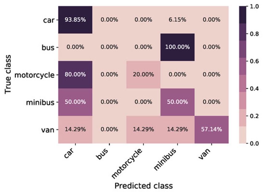
Figure 15. This classification matrix tracks the prediction accuracy of the standard transfer learning network when evaluated against actual sensor data, illustrating the distribution of correct and incorrect categorizations across all vehicle types and establishing a baseline success metric of 83.75%.
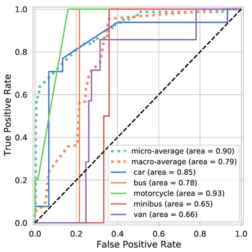
Figure 16. This line chart maps the true-positive versus false-positive rates for the standard transfer learning network across different detection thresholds, highlighting individual vehicle category performance when using physical sensor data.
In sharp contrast to both the standard paradigm and the dual-stage enriched strategy, the synthetic TL variant—denoted by the red boundary in Figure 3—is optimized using virtual data alone before being subjected to direct testing on the empirical LiDAR test suite.
The classification behavior of this synthetic-trained COCO Faster RCNN design is cataloged via the confusion matrix in Figure 17 and the performance curve in Figure 18. This framework reached an overall classification accuracy of 61.25% alongside an F1 metric of 0.605 on the physical test sequence. Analysis of the errors reveals that a substantial portion of misclassified passenger cars are erroneously tagged as commercial buses, a phenomenon that occurs predominantly when the sensor captures only a single isolated edge of the vehicle profile.
Additionally, the system displays poor recognition of motorcycles, which stems from the geometric profile differences for two-wheeled vehicles between the virtual generation environment and physical environments. Conversely, the model achieves error-free prediction for the bus category, yielding an AUC of 1.0 as traced by the orange trend line in the performance curve of Figure 18. This perfect score is likely an isolated artifact tied to the low total volume of buses within the evaluation pool (the constrained sample size also explains the distinct stair-step pattern of the tracking line).
Beyond this exception, the generalized metrics fall well below the standard TL setup, producing micro- and macro-averaged AUC statistics of 0.74% and 0.68%, respectively. Furthermore, multiple classes—specifically passenger cars, motorcycles, and minibuses—demonstrate nearly zero discriminative separation, though the network does successfully retain a baseline level of structural information.
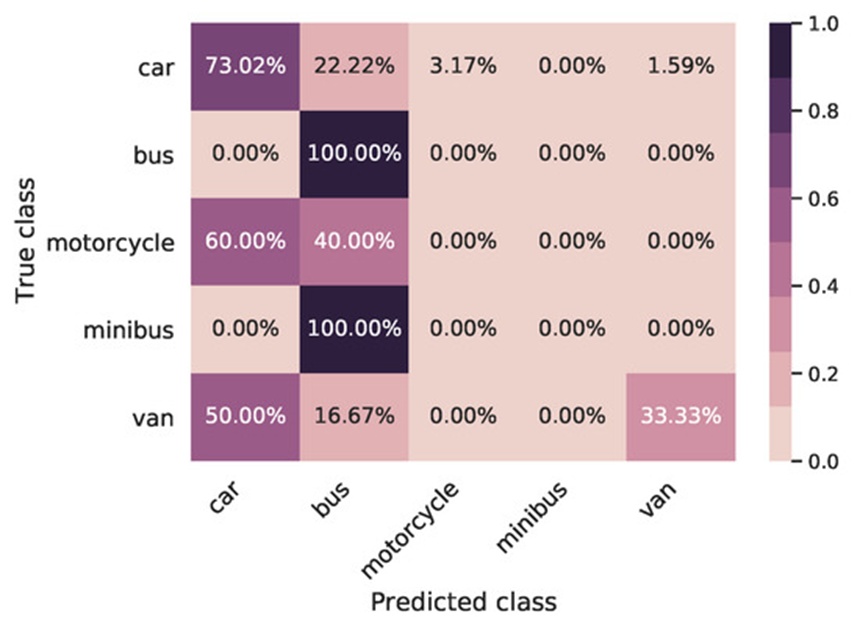
Figure 17. This evaluation matrix maps the identification accuracy and error trends of the model trained exclusively on generated virtual data, illustrating its specific classification weaknesses and its 61.25% correct prediction rate when confronted with real sensor inputs.
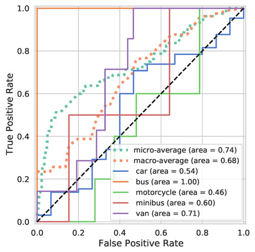
Figure 18. This performance plot traces the sensitivity and specificity of the virtual data model, demonstrating a segmented, stair-step profile due to restricted real-world test targets and showing an isolated perfect score for large transit vehicles.
This subsection evaluates a dual-stage optimization pipeline that blends virtual data with empirical samples to determine whether synthetically generated shapes can inject useful discriminative properties into the classification network. The complete pipeline for this synthetically enriched strategy is diagrammed in Figure 3. Two distinct transfer learning protocols are evaluated below: frozen feature extraction and active weight optimization.
Initially, we consider the outcomes of the frozen feature extraction pipeline. This protocol treats the internal layers of the synthetic TL variant as a fixed feature selector, locking all upstream weights while updating only the final softmax classification layer using physical target data. This setup secured an overall classification accuracy of 86.25% alongside an F1 score of 0.872 when run against the real-world LiDAR test suite. Encouragingly, these values exceed the metrics of the standard TL approach. However, because the active weight optimization pipeline yielded even higher performance while exhibiting a nearly identical error distribution, its specific operational metrics are emphasized below.
The active weight optimization protocol unfreezes the entire model architecture, allowing all layers to adapt to the physical LiDAR training samples under a suppressed learning rate to maximize decision boundaries. The resulting metrics for this dual-stage framework are mapped in the confusion matrix found in Figure 19 and the performance curves shown in Figure 20.
The framework attained an overall classification accuracy of 91.25% and an F1 score of 0.906 on the actual LiDAR test set. These values confirm that unfreezing the structural layers allows for more precise class resolution than is possible through a standard single-stage transfer learning routine.
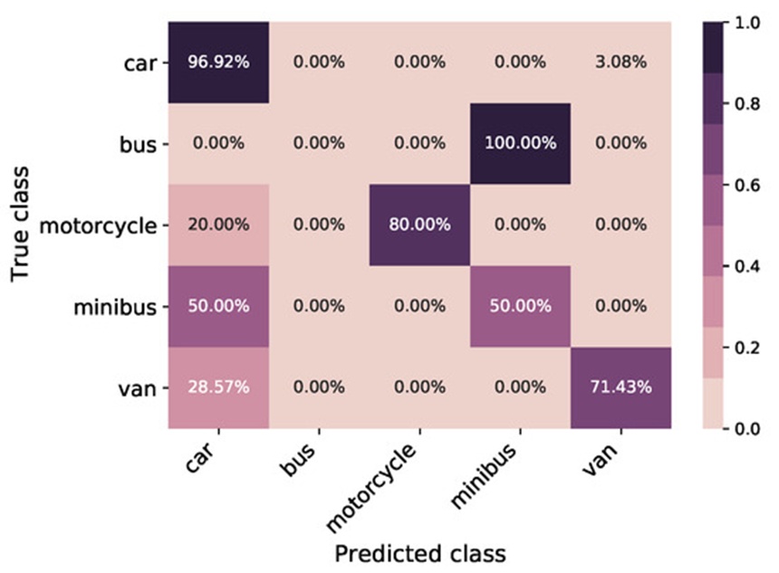
Figure 19. This performance matrix displays the classification accuracy achieved by combining synthetic and actual data through full network retraining, highlighting a significant reduction in class confusion and a peak success rate of 91.25%.
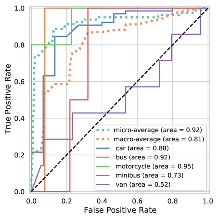
Figure 20. This sensitivity chart plots the true-positive classification rates for the dual-stage retraining model, illustrating an upward shift in detection curves across nearly all vehicle types.
In the accompanying performance curves, all individual vehicle classes demonstrate strong metrics except for the Van category, an outcome tied directly to the limited volume of physical examples available during the second-stage refinement. Both the micro and macro average metrics show clear upward trends, which is mirrored by the individual AUC metrics for Cars, Motorcycles, Minibuses, and Vans relative to both the purely synthetic and standard single-stage configurations.
While the absolute AUC boundary of this dual-stage method remains close to the standard TL approach, the structural shape of the curves and the overall error rates reveal a major shift, in accordance with the definitions in [58]. Compared to the baseline standard TL model, this configuration suppresses the classification accuracy error rate by 46.15% and decreases the F1 score error by 40.81%, showing a clear performance advantage.
Table 3 provides a consolidated breakdown of all examined models run against the physical LiDAR data, tracking classification accuracy, weighted F1 metrics, mean Intersection over Union (IOU), IOU variance, and total processing duration.
With the exception of the purely synthetic setup, all models present uniform values for both mean IOU and its associated variance. Processing times also remain consistent across the board, save for the purely synthetic framework, which requires significantly longer training periods because it scales to a much larger synthetic data array. Overall, this dual-stage framework provides an increase in F1 score capability of 7.5% relative to the standard TL pipeline. A visual confirmation of the actual targets identified within the LiDAR point cloud using our dual-stage weight modification pipeline is presented in Figure 21.
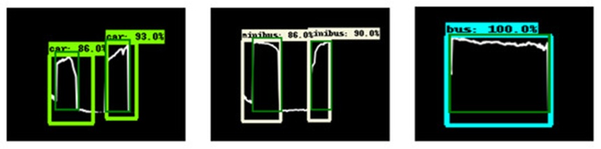
Figure 21. This visualization provides a spatial breakdown of real-world point cloud detections, demonstrating the practical bounding box alignment and geometric overlap achieved by the dual-stage retraining approach.
Table 3. This structured dataset provides a comparative overview of all evaluated models, highlighting accuracy metrics, overlap statistics, and processing times while documenting how the dual-stage framework minimizes errors compared to standard transfer learning setups.
Model | Processing Time | IoU Variance | Mean IoU | F1-Based Error Reduction | F1-Score | Error Reduction Relative to Baseline | Classification Accuracy |
Classic Transfer Learning (CTL) | 688.006 s | 0.272 | 0.418 | N/A | 0.837 | N/A | 83.75% |
Synthetic Transfer Learning Model | 17,250 s | 0.211 | 0.252 | −58.06% | 0.605 | −58.73% | 61.25% |
Synthetic-Augmented Transfer Learning (Weight Reuse) | 693.86 s | 0.273 | 0.520 | 40.81% | 0.906 | 46.15% | 91.25% |
Synthetic-Augmented Transfer Learning (Feature Extraction) | 688.01 s | 0.263 | 0.494 | 26.5% | 0.872 | 36.3% | 86.25% |
To statistically confirm the performance gains of the synthetically enriched TL framework over the standard single-stage TL framework, we evaluated the following hypotheses at a significance threshold of \alpha = 0.05:
Null Hypothesis H_0: There is no measurable performance variation between the synthetically enriched TL framework and the standard TL framework.
Alternative Hypothesis H_1: The synthetically enriched TL framework achieves a higher level of performance than the standard TL framework.
Applying a Chi-square independence test across both test pools using the respective F1 scores produced a Chi-square statistic of 3.89, yielding a corresponding p-value of 0.048. Because p < 0.05, the null hypothesis is rejected in favor of the alternative hypothesis, confirming that the synthetically enriched TL framework provides a statistically significant improvement in classification capability over the standard TL model.
This paper has presented an original methodology for roadside vehicle identification utilizing a synthetically enriched transfer learning pipeline tailored for LiDAR point clouds. A computationally lean simulation utility was built to generate synthetic LiDAR data, leveraging the extensive collection of three-dimensional vehicle models available in the ShapeNet repository combined with ray casting techniques to emulate physical sensor behavior. The resulting dataset provides rich geometric diversity and varying environmental constraints, making it an excellent proxy for actual LiDAR data when field samples are difficult to obtain.
Furthermore, detailed experimentation demonstrates that our dual-stage transfer learning pipeline markedly improves object detection performance, cutting the classification accuracy error by 46.1% and reducing the F1 score error rate by 40.81% relative to the traditional transfer learning baseline. While prior work has paired transfer learning with simulated data across other domains, to our knowledge, this represents the first viable, economically sustainable application optimized for LiDAR sensors or utilizing virtual data amplification for vehicle tracking and classification.
The structural workflow was thoroughly tested on real-world LiDAR data streams and cross-validated using camera images. This methodology enables the rapid deployment of object recognition networks in environments where precisely labeled physical samples are scarce, offering a scalable template for constructing cost-effective, LiDAR-based parking management infrastructures.
Upcoming research will focus on a sensitivity analysis to isolate how individual variations within the simulated data affect overall network accuracy. Additional work will target maximizing the computational efficiency of the optimization phase to minimize the time required to deploy these networks effectively across varied geographical environments.
The authors would like to thank: Innovate UK for funding the work on the PARSER project; Vortex IoT, the lead on the PARSER project, for the opportunity to collaborate on the work; collaborators on the project—British Telecommunications Plc and Swansea and City Council—for their contributions; and all the people in the wider team for creating a fun and enjoyable working environment. The authors would like to acknowledge the UK Engineering and Physical Sciences Research Council (EPSRC) (EP/S001387/1; EP/V061798/1). The authors also would like to acknowledge the Ser Cymru Infrastructure Grant, AccelerateAI, part-funded by the ERDF via the Welsh Government.
None
This research was funded by Innovate UK grant number 23634.
None
Open Access The author(s) retain copyright. This article is licensed under the Creative Commons Attribution-NonCommercial-ShareAlike 4.0 International License. It may be shared and adapted for non-commercial purposes with appropriate attribution, an indication of changes, and distribution of adaptations under the same license. Third-party material may be subject to separate terms identified in its credit line. View the license at https://creativecommons.org/licenses/by-nc-sa/4.0/.
 Transparent Intelligence Publishing