The pressing issue of adversarial vulnerability in classifiers, particularly those implemented via deep neural networks, is examined. This problem is investigated through a generalization applicable to any classification models generated by machine learning techniques. The insufficiency of conventionally accepted metrics for evaluating classifier quality is highlighted, including metrics deployed to validate the efficacy of defense mechanisms against adversarial manipulation. The underlying causes behind the generation of adversarial examples and other machine learning-based classification errors are explored. A methodology for simulating adversarial attacks is introduced, demonstrating the core phenomena encountered during such exploits. The necessity of establishing quality metrics specifically tailored to quantify potential classifier vulnerability to adversarial threats is emphasized. To evaluate robustness against adversarial interference, the application of the multidimensional EDCAP metric (Excess, Deficit, Coating, Approx, Pref) is proposed. Furthermore, a technique is presented for constructing a novel multiclass classifier, termed EnAE (Ensemble of Auto-Encoders), which leverages an ensemble of single-class classifiers governed by the EDCAP evaluation criteria. The EnAE classification framework employs a hard voting mechanism and is capable of identifying anomalous input data. The introduced metric, construction framework, and classifier are validated across multiple datasets characterized by feature spaces of moderate dimensionality.
Adversarial attacks represent intentionally crafted inputs designed to induce decision errors in machine learning-based classifiers. Historically, adversarial instances have been characterized by their minimal mathematical divergence from properly classified data points [1]. Broadly speaking, however, the geometric proximity of these instances becomes secondary if the system unpredictably reaches a conclusion fundamentally distinct from the decision a human operator would make in an identical context.
Given the pervasive deployment of machine learning architectures and their derivative classifiers, malicious actors frequently exploit these vulnerabilities to launch targeted disruptions against artificial intelligence systems. The most exposed frameworks are intelligent models engineered for image and voice recognition; nonetheless, exploitation can similarly target classifiers operating on network traffic, digital files, discrete events, and natural language text. To compromise these systems, adversaries alter the incoming data stream by introducing image distortions, injecting noise into network data flows, adjusting file structures, manufacturing distracting events, or altering text strings. Well-documented instances of real-world compromises include exploits targeting voice assistants—such as executing unauthorized purchasing transactions via Amazon Alexa [2]—and bypassing spam filtration protocols [3]. Multiple production-grade classification systems are known to be vulnerable to adversarial manipulation, notably computer vision models [4-6], facial verification systems [7], and related frameworks [8]. These and other instances of faulty execution in artificial neural networks prevent full reliance on these technologies within operational domains where errors carry high liabilities. A prime example is the autonomous driving system in Tesla vehicles, where classification failures within the autopilot mechanism generated significant publicity due to their severe real-world outcomes [9]. The susceptibility of the computer vision pipeline utilized by Tesla to adversarial exploitation had been previously established by independent investigators [10-12].
The erratic behavior displayed by machine learning frameworks highlights the urgency of establishing robust defensive measures for classifiers against adversarial exploits. Concurrently, defensive methodologies remain far from completely realized or comprehensively mapped. A majority of existing countermeasures rely on heuristic approaches that fail to guarantee consistent classification performance across general machine learning applications. Furthermore, standardized protocols for measuring a trained classifier's vulnerability level to adversarial vectoring are missing, preventing systematic comparisons between different models.
In this study, the fundamental drivers behind classifier susceptibility to adversarial attacks are analyzed, and a novel multidimensional evaluation metric, EDCAP, is introduced to provide a quantitative measure of this vulnerability. The generalized model formulated herein accounts for the primary phenomena documented in empirical studies. These phenomena encompass the feasibility of executing adversarial vectors under both white-box and black-box access constraints, alongside the vulnerability of diverse machine learning paradigms, including neural networks, support vector machines (SVMs), and decision trees. Additionally, a new paradigm for synthesizing a multiclass classifier utilizing an ensemble of single-class neural network auto-encoders is presented, giving operators control over classification quality and yielding enhanced resilience against adversarial manipulation. The utility of this methodology is benchmarked against standard multiclass classification systems using the publicly accessible multidimensional datasets “Fisher’s Irises” [13] and “Wheat Seeds” [14]. The capacity to quantitatively measure adversarial susceptibility via the EDCAP parameters is verified.
Our core contributions are twofold:
The introduction of a novel multidimensional quality metric, EDCAP, for multiclass classification systems.
The design of a new synthesis framework for the EnAE multiclass classifier constructed from an ensemble of single-class models.
The primary benchmark for evaluating machine learning success in image classification centers on minimizing empirical error across a designated training set. However, a seminal study [15] demonstrated that deep neural networks exhibit highly erratic classification behavior within the immediate vicinity of training data points, yielding highly counterintuitive outcomes. This research coined the term “adversarial example” to describe input patterns that exhibit negligible deviations from training samples yet trigger entirely unexpected classification outputs.
Subsequent research [1] delved into the underlying mechanics of adversarial instances within deep neural network topologies, presenting straightforward techniques for engineering adversarial data. The investigators concluded that the presence of adversarial vulnerabilities in neural network-based classifiers stems primarily from their inherently linear characteristics.
Following these foundational discoveries, a broad research community emerged to address the identification of adversarial examples and the formulation of resilient protective strategies.
At present, an array of frameworks has been engineered to automate the generation of adversarial instances. Certain techniques operate under full visibility of the target classification architecture (white-box conditions). Notable examples within this category include the fast gradient sign method (FGSM) [16], the Jacobian-based saliency map approach aimed at isolating the most influential pixels for a classification choice [17], and the Carlini–Wagner optimization attack [18]. Conversely, when the internal parameters of the classification framework are hidden (black-box conditions), alternative mechanisms are deployed, such as substitute model attacks [19], single-pixel perturbations [20], and generative adversarial network (GAN)-based strategies [21]. While these specific methodologies were explicitly formulated for image domains, their core mathematical paradigms translate to alternative data modalities. Additionally, specialized software suites for executing adversarial evaluations have been introduced, including ART-IBM, FoolBox, CleverHans, ALFASVMlib, AdversariaLib, and MLsploit.
To mitigate adversarial risks in deep neural networks, multiple strategies have been investigated, including substituting standard activation functions with Bounded-RELU variants [22], implementing adversarial training regimes [23], utilizing defensive distillation protocols [24], and executing feature squeezing mechanisms [25]. These protective methodologies share systemic limitations: they fail to offer comprehensive immunity across all attack vectors, increase computational overhead during training, and frequently degrade baseline accuracy. Furthermore, the secondary neural architectures integrated into certain defensive schemes behave as uninterpretable black boxes themselves. Although numerous empirical evaluations of modern defensive toolkits have been documented [26], showing a reduction in the success rate of adversarial interventions [27, 28], separate research endeavors focus on analyzing intrinsic data traits to establish identification benchmarks for isolating adversarial inputs [29].
An examination of current literature indicates that a universally accepted and universally effective countermeasure against all variants of adversarial exploits remains unavailable. Indeed, certain studies [30] argue that under high-dimensional data regimes, the vulnerability of multilayer neural network configurations to adversarial manipulation becomes structurally unavoidable.
The performance of defensive strategies against adversarial vectors is conventionally quantified via the probability of successfully identifying adversarial instances:
“The study shows that defensive distillation can reduce the effectiveness of sample creation from 95% to less than 0.5% on a studied DNN” [24],
“The results showed that our defending method achieved up to 96.3% classification accuracy on black-box adversarial examples, and detected up to 98.7% of the high confidence adversarial examples” [31],
“The proposed method achieves 65% to 100% accuracy detecting adversarials with a wide range of attacks” [29].
In these instances, empirical probability assessments are typically bounded by the specific adversarial generation techniques applied against a classifier trained on a particular dataset. Consequently, the computed vulnerability metric of a classification model depends directly on both the specific classifier architecture and the particular algorithm used to construct the adversarial samples. This dependency prevents the derived numerical score from being interpreted as an intrinsic quality metric of the classifier itself, independent of the attack methodology.
Concurrently, relying solely on classical classification performance metrics derived from the confusion matrix—such as accuracy, precision, recall, and F-score—fails to uncover the operational characteristics of the classifier when exposed to inputs outside the boundaries of the training and validation datasets.
A remarkable property of adversarial examples is their cross-model transferability across different architectures implementing the target classifier [32]. Notably, the underlying models executing the classification can feature entirely distinct structural paradigms; for instance, one system may utilize a deep neural network while another relies on a Support Vector Machine (SVM). This characteristic, combined with the capability to engineer successful adversarial patterns without direct access to the internal parameters of the target model (black-box conditions), strongly indicates that the root cause of adversarial vulnerability resides within the underlying data distribution used to train the classifier.
Historically, it was observed in [1] that the emergence of adversarial vulnerabilities is largely driven by the linear behavior of classifiers when confronting highly non-linear problems solved by modern machine learning techniques. Currently, the research community is predominantly focused on investigating deep neural network architectures. As a consequence, the phenomenon of adversarial vulnerability is routinely linked with deep neural networks, which diverge significantly from linear frameworks. However, it remains clear that the presence of adversarial vulnerabilities can be readily demonstrated within less complex network topologies, such as a multilayer perceptron.
To illustrate, consider the outcome of mapping the feature space across an extended neighborhood surrounding the training data region of a neural network auto-encoder configured as a single-class classifier (Figure 1). Under this setup, a significant volume of coordinates situated far from the training sample domain are erroneously categorized as positive. In addition to establishing a valid classification envelope around the training samples, the neural network inadvertently generates an isolated, erroneous decision zone separated from the primary data cluster. Any sample falling within this detached envelope is improperly assigned to the target class. This visualization underscores that adversarial instances can manifest within simple neural architectures as a direct byproduct of their non-linear characteristics.
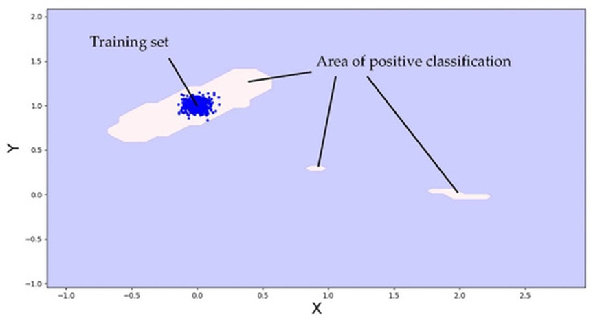
Figure 1. Areas of classification of the neural network auto-encoder.
It is essential to systematically analyze how adversarial instances emerge across conceptually diverse classification paradigms, including multilayer neural networks and SVMs. Throughout this process, it is preferable to minimize reliance on intricate adversarial generation algorithms. This independence enables an objective assessment of classifier quality that is decoupled from any specific attack optimization method. Furthermore, such foundational research does not strictly require high-dimensional benchmarks, such as the MNIST or CIFAR image repositories.
The design of classification systems resilient to adversarial manipulation necessitates a well-defined, quantitative quality metric. Formulating such a standardized benchmark is expected to simplify both the engineering of adversarial-hardened frameworks and the direct comparison of competing classifier models.
The majority of machine learning techniques used to build classifiers suffer from inherent limitations arising from the requirement to construct a computable decision boundary from datasets that are frequently unbalanced in terms of sample size and spatial density. To mitigate this, alternative strategies leverage ensembles of classifiers to make collective decisions [33], including ensembles composed of single-class models [34]. Generally, a consensus voting strategy is deployed across diverse classifier models, as detailed in [35], yielding a more stable decision boundary than any individual classifier can provide. For multiple operational reasons, adapting this multi-model paradigm holds significant promise for engineering classification systems with mathematically verifiable resistance to adversarial exploits.
It is evident that despite the extensive body of literature analyzing adversarial vulnerabilities, a standardized method for the quantitative evaluation of classifier quality from a security-robustness perspective has not yet been established. Developing and validating an evaluation framework suitable for cross-model benchmarking remains a critical priority.
Furthermore, academic literature reveals that current approaches for synthesizing adversarial-hardened classifiers predominantly rely on regularization techniques aimed at inducing more robust learning boundaries, which nonetheless fail to guarantee the target security properties under generalized conditions. Additionally, empirical validation of adversarial resilience typically relies on specific, localized attack generation techniques, which cannot provide an exhaustive map of the classifier's behavioral envelope.
Throughout the remainder of this paper, the mathematical notation and terminology summarized in Table 1 are utilized.
Table 1. Designations.
Symbol | Description |
𝑋 | A feature space representing a set of objects to be classified, which may be uncountable |
|𝑋| | 𝑋 |
𝑋𝑇, | A training subset containing all objects |
A training subset containing all objects belonging to class 𝑖 | |
𝑇 | A discrete (countable) subset typically used as the training set in standard machine learning settings |
A test subset consisting of all objects assigned to class 𝑖 | |
𝑋𝐷 | The set of objects classified as positive by a one-class classifier |
The set of objects classified as members of class 𝑖 | |
𝑋𝑆 | A structured N-dimensional grid of points defined over a restricted subset of 𝑋 |
Training samples projected onto their nearest corresponding grid points in 𝑋𝑆 | |
A subset of grid points in 𝑋𝑆 that are classified as positive | |
ϒ | The collection of class labels |
𝐶L1 | A one-class classification model |
𝐶LK | A multi-class classifier that assigns an input to one of K class labels |
𝐶LO | A binary classifier indicating whether an object belongs to any predefined class (1) or not (0) |
𝐶L(i) | A class-specific classifier for class 𝑖, outputting 1 if the object belongs to class 𝑖, otherwise 0 |
𝐴E0 | An autoencoder trained to assess membership across all labeled classes collectively |
𝐴E(i) | An autoencoder specialized for determining membership in class 𝑖 |
𝑁𝑁𝑛,ℎ1,…,ℎ𝑘,𝑚 | A neural network architecture with 𝑛 input nodes, 𝑚 output nodes, and hidden layers containing ℎ1,…,ℎ𝑘 neurons across 𝑘 layers |
𝑅𝐸 | Reconstruction error used as a measure of discrepancy in an autoencoder’s output |
Let us formulate the problem of building a classifier via machine learning protocols. For analytical simplicity, we focus on a one-class classification scenario. Let Content denote the domain of objects to be classified, where X represents the set of classified objects. For a single-class classification model, the output space is defined as 𝑌={0,1}, where 1 denotes target class alignment and 0 denotes non-alignment. The specific subset containing target class elements is represented as 𝑋𝑇⊂𝑋. Let us define the ideal object membership function for this target category as:
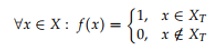 (1)
This function represents an optimized, flawless single-class classifier; however, in empirical applications, collecting every valid coordinate 𝑥∈𝑋𝑇 for training purposes is generally unfeasible. Instead, we typically operate with a finite, countable training dataset 𝑇⊂𝑋𝑇, which serves to construct training patterns alongside independent subsets for validation and testing. Let the trained single-class classifier model be denoted as:
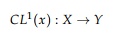 (2)
Even though 𝐶𝐿1 is optimized using the subset 𝑇⊂𝑋𝑇, the resulting model synthesis can yield multiple operational states corresponding to standard binary classification outcomes (Table 2): True Positive (TP), True Negative (TN), False Positive (FP), and False Negative (FN).
Table 2. Binary Classification Outcomes.
Classification\Class | 𝐍𝐞𝐠𝐚𝐭𝐢𝐯𝐞 𝒙∉𝑿𝑻 | 𝐏𝐨𝐬𝐢𝐭𝐢𝐯𝐞 𝒙∈𝑿𝑻 |
Positive | 𝐹𝑃: 𝐶L1(𝑥)=1 | 𝑇𝑃: 𝐶L1(𝑥)=1 |
Negative | 𝑇𝑁: 𝐶L1(𝑥)=0 | 𝐹𝑁: 𝐶L1(𝑥)=0 |
In practice, an empirical single-class classifier deviates from the ideal baseline function because the geometric boundary of the object set it labels as the target class undergoes distortion, meaning the classified space 𝑋𝐷 diverges from the true target space 𝑋𝑇:
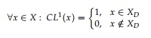 (3)
This spatial divergence can be conceptualized and visualized in Figure 2.
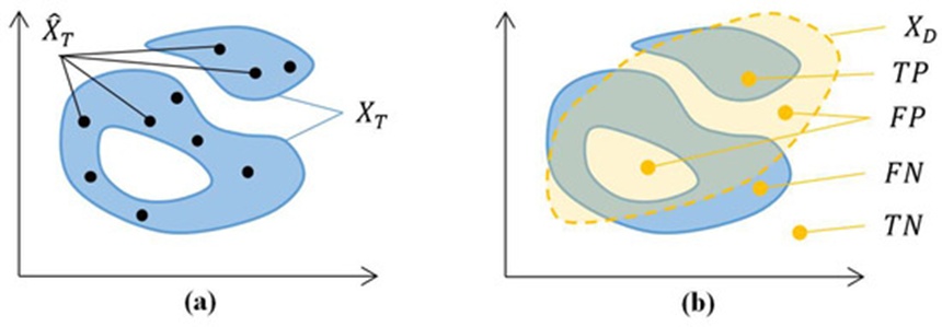
Figure 2. Target class area (a) and deformed area (b).
The intrinsic performance of a single-class classifier is determined by the mathematical proximity of 𝐶𝐿1 to the ideal operator f, which can be quantified by comparing the geometric properties of the set 𝑋𝐷 against 𝑋𝑇. Specifically, the error conditions FP and FN represent deviations from ideal performance. The FP condition emerges when 𝑋𝐷\𝑋𝑇≠∅, whereas the FN condition manifests when 𝑋𝑇\𝑋𝐷≠∅, where the operation\denotes signifies set subtraction. For continuous domains of classification points, we define spatial volume using the notation |X|, where |∅|=0. Consequently, the occurrence of FP and FN errors can be mathematically expressed in terms of volume as:
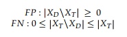 (4)
It is critical to note that the collection of adversarial examples targeting a single-class classifier maps directly to the set FP. Conversely, the domain of accurate positive classification is expressed volumetrically as:
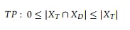 (5)
Furthermore, the condition |𝑋𝑇\𝑋𝐷|=0 naturally follows from the set intersection property 𝑋T∩𝑋D=𝑋T.
To ensure that the quantitative assessment of classifier quality remains unskewed by the baseline volume of the target set—thereby enabling objective performance comparisons across disparate domain applications—we introduce normalized quality metrics scaled to the volume of the target domain:
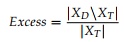 (6)
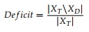 (7)
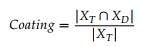 (8)
The metric Excess scales above 0 if 𝐶𝐿1 incorrectly assigns positive labels to objects residing outside the true target boundary. The Deficit metric ranges between 0 and 1; if 𝐶𝐿1 misclassifies authentic target objects as non-members, this value exceeds 0. The boundary condition Deficit=1 represents a complete failure mode where the true target domain and the classifier's predicted domain share no overlapping space. The Coating metric similarly spans from 0 to 1, where a value of 0 indicates a null intersection between 𝑋𝑇 and 𝑋𝐷 (an outcome highly improbable under any coherent machine learning training regime), while a value of 1 represents the standard successful training outcome where the classifier maintains correct decisions across the entire training space.
The geometric approximation accuracy of the target domain can be evaluated as the volumetric ratio of the true target space relative to the deformed space mapped by the classifier:
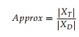 (9)
An ideal single-class classification system is characterized by the following deterministic quality metrics:

Aggregated together, these parameters construct a multidimensional evaluation framework designated as the EDCA criterion. This metric suite was originally introduced by the authors in [36] to provide a quantitative framework for evaluating the performance of anomaly detection models built on neural network auto-encoders.
In empirical settings, the data points comprising a training dataset are fundamentally discrete. To compute these proposed quality metrics for operational classifiers, it is necessary to implement a grid-based approximation of the continuous space, bounded by a defined workspace where the quality metrics are evaluated. By confining the space to a operational area that comprehensively encompasses both the training and testing data coordinates, we can normalize the spatial dimensions within a strict range from 0 to 1. We establish a uniform grid structure with a step size of h across all coordinates of this bounded space. Consequently, for an N-dimensional feature space, the system generates () discrete grid cells. This total collection of cells is defined as the scan set X_S. The coordinate points belonging to the sets 𝑋𝑇 and 𝑋𝐷 are then mapped directly to their corresponding spatial cells within the scan set. Through this discretization, the training data points populate the subset ⊂𝑋𝑆, while the subset ⊂𝑋𝑆 is populated by cells whose central coordinates yield a positive classification decision from the model.
It is recommended to calibrate the cell resolution h relative to the dataset under analysis such that the density of training samples within each individual cell balances and approaches 1. Setting an excessively fine cell resolution under high-dimensional data regimes exponentially increases computational overhead. Furthermore, an overly small value for h can cause adjacent points in 𝑋𝑇 to become isolated from one another in the scan set by a sequence of unpopulated cells not contained within the true distribution, which risks undermining the mathematical validity and stability of the numerical EDCA metrics.
An illustrative example mapping the numerical EDCA evaluations for an isolated single-class classifier is provided in Figure 3.
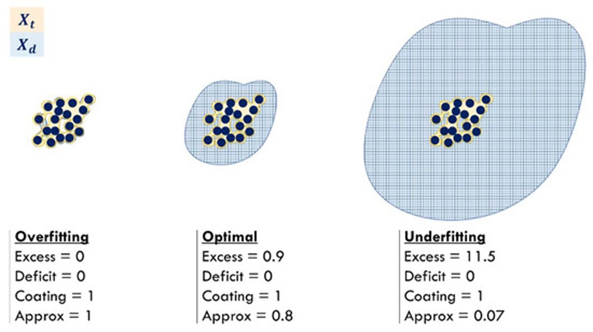
Figure 3. The relationship between the size of the area and the values of the EDCA characteristics.
The metrics Deficit and Coating primarily define classification performance within a traditional framework. Conversely, the Excess attribute is crucial for evaluating how susceptible a model is to adversarial manipulation. This metric quantifies the volume of the positive classification region within the feature space that extends beyond the perimeter of the training dataset. As illustrated in Figure 3, a larger region corresponds directly to an increased Excess value. By evaluating the Excess metrics across various models, researchers can quantify and compare adversarial risks based on the volume of the feature space capable of containing error-inducing samples. Notably, determining Excess requires no internal knowledge of the model architecture (operating under a black-box paradigm), which enables the comparison of highly diverse classification mechanisms.
The Approx metric indicates the degree of alignment between the positive classification zone and the training data. When a classifier exhibits high permissiveness and low robustness against adversarial vectors, its Approx value approaches 0. It is worth highlighting that even an "ideal" model operating at optimal metric thresholds remains susceptible to false negative (FN) errors if the underlying training data is non-representative. Such misclassifications can conceptually be categorized as a form of adversarial vulnerability. Furthermore, if the operational context dictates that false positive (FP) errors carry greater severity than type II errors, selecting a model that minimizes the Excess parameter is advisable.
As previously established, conventional performance metrics derived from a confusion matrix are insufficient for comprehensively evaluating the behavior of machine learning-driven classifiers. To properly evaluate model resilience against adversarial disruption, this study proposes investigating the behavioral patterns of the trained model within the feature space regions adjacent to the training data. This evaluation framework can be demonstrated using a classifier trained on a dataset 𝑋𝑇 containing M distinct classes. Let represent the subset of training samples associated with class i, where 𝑖=. Correspondingly, the set of instances assigned to class i by the trained model is designated as .
To quantitatively assess the attributes of a multiclass model, a multidimensional EDCA framework can be applied, which aggregates the previously defined metrics across individual classes. Under this approach, distinct metrics including Excess(i), Deficit(i), Coating(i), and Approx(i) are determined for each class. This diagnostic criterion was initially introduced to measure the performance of models designed for dynamic classification amid concept drift [37], and it has been formally analyzed alongside traditional confusion matrix metrics [38].
A defining attribute of multiclass environments is the partial overlap between regions enclosing instances from different classes, a phenomenon exemplified by the Iris dataset [13]. In such scenarios, establishing a theoretically flawless classifier is inherently unfeasible, an established reality within machine learning research.
Data ambiguity within the training set is identified by a non-zero intersection between the domains of classes i and j:
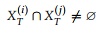 (10)
Within this region of ambiguous definition, any given sample functions as an adversarial instance to some extent. To appraise model behavior within these ambiguous zones, one can quantify its preference 𝑃(𝑖) for a specific class relative to the remaining categories. For a two-class intersection, this preference metric can be formalized as the ratio of the volume where the model assigns membership to a specific class to the total volume of the overlapping ambiguous domain:
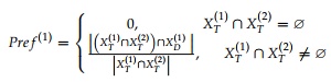 (11)
The spatial representation of this preference region is illustrated in Figure 4.
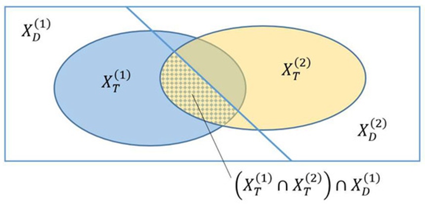
Figure 4. Example of a Class 1 preference area in the ambiguity region (∩) ∩ .
Extending this definition to accommodate the overlapping domains of multiple classes yields:
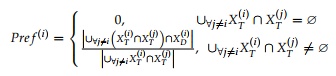 (12)
The metric Pre(i) scales from 0 to 1, indicating the model's propensity to decide in favor of class i within ambiguous regions. For operational deployment, this metric must be computed across the cells of the scanning grid .
Consequently, to provide a comprehensive numerical profile of a multiclass system, it is recommended to evaluate Excess(i), Deficit(i), Coating(i), Approx(i), and Pref(i) for every class.
Relying on an evaluation metric whose dimensionality scales with the number of classes can be impractical. However, assuming uniform importance across all classes, a 5-tuple comprising Excess, Deficit, Coating, Approx, and Pref serves as a robust quantitative performance baseline, where each element represents the worst-case performance across all classes:
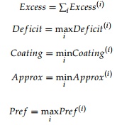 (13)
For the Deficit, Coating, Approx, and Pref components, the most unfavorable bound (the minimum or maximum) is selected, whereas the global Excess is determined by summing the values across all classes. This aggregated set of metrics establishes the multidimensional EDCAP evaluation framework, enabling model comparison while accounting for potential class domain intersections. Computing these EDCAP parameters requires utilizing an identical scanning set XS, maintaining a uniform operational space and grid resolution.
Assuming an adversarial attack targeting class i is defined as an exogenous sample misclassified into class i, the metric Excess(i) serves as the primary indicator of vulnerability. Nonetheless, in scenarios featuring overlapping class boundaries, evaluating Pref(i) becomes equally essential.
Under these conditions, evaluating the relative adversarial vulnerability of two classifiers simplifies to comparing their computed Excess parameters, provided the training sets do not overlap. The model that exhibits a minimized Excess metric possesses a smaller spatial footprint susceptible to generating adversarial errors across all categories.
Consider the challenge of designing a classification system that exhibits robust resistance to adversarial threats. To measure this robustness, the EDCAP diagnostic framework is utilized. Initially, it is vital to evaluate the structural properties of standard classifiers built using traditional machine learning techniques. For this purpose, the analytical framework employed for calculating EDCAP performance indicators is highly effective, as it permits the spatial visualization of decision boundaries across all categories. Typical configurations of these decision boundaries are illustrated in Figure 5.
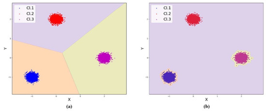
Figure 5. The first (a) and second (b) feature space separation variant of machine learning classifiers.
These conventional methods of partitioning the feature space post-training serve as a primary source of model vulnerability. For instance, in the scenario depicted in Figure 5a, any given sample—regardless of its distance from the true boundary established by the training set—will be assigned to that specific category. Deploying a model with such characteristics is highly problematic for critical applications, such as network intrusion detection. In the case shown in Figure 5b, sample instances located near the true boundaries of class Cl.1 and class Cl.3 are erroneously assigned to class Cl.2. Consequently, the model in Figure 5b is susceptible to adversarial manipulations that induce false positive errors for classes Cl.1 and Cl.3, alongside false negative errors for class Cl.2. Utilizing this type of system in domains like computer vision or autonomous driving can precipitate severe outcomes due to erroneous decision-making.
These vulnerabilities can be mitigated by utilizing an ensemble configuration of auto-encoders for classification tasks. During the training phase, each individual auto-encoder aims to construct a tightly bounded topological region that encompasses the majority of the training points belonging to its target class. Let us formalize a multiclass classification system constructed from an ensemble of these auto-encoders. Every constituent auto-encoder is optimized exclusively on the samples of its assigned class; instances from any other class are treated as anomalies. The primary characteristic of an auto-encoder is its minimal reconstruction error when processing samples from its training distribution or close variants thereof. Conversely, an elevated reconstruction error signals that the model did not encounter similar data during training. To distinguish recognized data patterns from novel or anomalous inputs, a reconstruction error threshold RE_{th} is applied, establishing the system's sensitivity to novelty.
In addition to class-specific models, it is advantageous to integrate a global auto-encoder AE_0. This unit differentiates known class profiles from exogenous inputs that do not resemble any of the recognized categories. Operating as an anomaly detection layer, this model provides a secondary perimeter of defense against adversarial vectors.
An example of this feature space partitioning achieved via an ensemble of neural network-based auto-encoders is displayed in Figure 6.
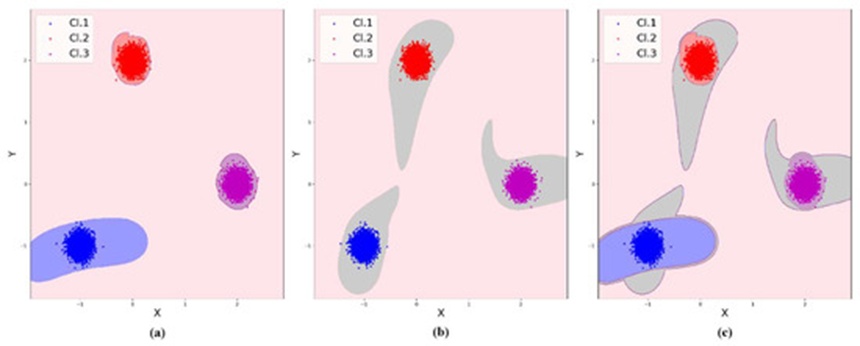
Figure 6. Feature space separation after training an ensemble of auto-encoders: specific class auto-encoders (𝑖) (a), all classes auto-encoder 𝐴𝐸0 (b), combined effect of all auto-encoders (c).
Let us compute the EDCAP metrics for this illustrative scenario across three distinct classifier designs, including the ensemble configuration integrated with the global auto-encoder. Because this specific dataset contains no spatial overlap between class definition zones, the Pref metric remains zero.
The individual class values for the Excess and Approx indicators are compiled in Table 3.
Table 3. Excess and Approx values for individual classes.
Variant of the Classifier | Approx |
|
| Excess |
| s |
Cl.3 | Cl.2 | Cl.1 | Cl.3 | Cl.2 | Cl.1 | |
0.04 | 0.05 | 0.06 | 20.86 | 20.49 | 16.09 | |
0.71 | 0.02 | 0.74 | 0.40 | 54.13 | 0.36 | |
0.66 | 0.71 | 0.22 | 0.53 | 0.43 | 3.51 | |
Figure 6 (for all classes) | 0.27 |
|
| 2.72 |
|
|
An aggregated evaluation of these classification systems based on the EDCA metric suite is summarized in Table 4.
Table 4. EDCA Quality Characteristics for the Considered Classifiers.
Variant of the Classifier | Approx | Coating | Deficit | Excess |
0.04 | 1 | 0 | 57.44 | |
0.02 | 1 | 0 | 54.53 | |
0.24 | 1 | 0 | 4.86 | |
Figure 6 (for all classes) | 0.36 | 1 | 0 | 1.75 |
The compiled data clearly indicates that conventional classification models yield the highest Excess metrics, translating to elevated vulnerability to adversarial manipulation. This finding confirms the preliminary conclusions drawn from the visual inspection of Figure 5.
Another critical finding is the enhanced adversarial resilience demonstrated by the auto-encoder ensemble. Furthermore, this robustness can be systematically augmented by incorporating a shared, global auto-encoder optimized on the combined data from all constituent classes.
This section outlines the architecture, execution flow, and optimization methodology for the EnAE (Ensemble of Auto-Encoders) multiclass framework based on neural network architectures. This configuration embeds a global auto-encoder optimized on the union of all training categories, which empowers the system to identify inputs that fail to align with any known class definition. By controlling the classification boundaries beyond the training dataset using the EDCAP metric system, the resulting model achieves superior resilience against adversarial exploits.
Let us establish the foundational mathematical notation and definitions.
To denote a multilayer perceptron neural network architecture featuring n input units, fully connected hidden layers containing ℎ1,…,ℎ𝑘 neurons, and an output layer of dimensionality m, we apply the following formulation:
 (14)
To explicitly represent the integration of a Dropout layer, the letter D is incorporated into the structural expression:
 (15)
An auto-encoder is defined as a multilayer perceptron architecture where the input and output dimensions are identically equal to n, containing more than one internal hidden layer:
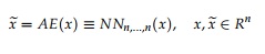 (16)
The operational output of the auto-encoder is quantified as the reconstruction error (RE):
 (17)
For data points belonging to the training distribution or proximate topologies, this reconstruction error must remain minimal, whereas it scales up for out-of-distribution inputs. The optimization of the auto-encoder over the training dataset 𝑋𝑇 is driven by minimizing this reconstruction metric:
 (18)
Establishing a reconstruction error threshold 𝑅𝐸𝑡ℎ allows for the implementation of a binary decision rule for a single-class classification framework:
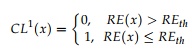 (19)
One viable approach to define this threshold value relies on identifying the maximum reconstruction error yielded across the training observations:
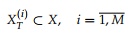 (20)
Let there be M discrete classes defined within the vector domain 𝑋⊆ , represented by their respective training subsets:
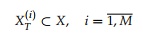 (21)
For analytical convenience, we introduce the unified training set encompassing all available classes:
 (22)
Assume there are corresponding testing evaluation subsets for each category:
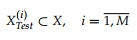 (23)
It is assumed that the datasets and have undergone all requisite preprocessing and feature normalization protocols.
The objective is to synthesize a composite classifier EnA(x) that assigns a class label i for any input 𝑥 ∈ 𝑋 if x aligns with the structural characteristics of , or returns 0 if x shows no similarity to any recognized class profiles.
The systematic optimization sequence for constructing the EnA(x) classifier is structured as follows:
Define the internal structural configurations for 𝐴𝐸0,𝐴𝐸(𝑖), 𝑖=
Execute the optimization phase for the neural network auto-encoders:
𝑇𝑟𝑎𝑖𝑛𝑖𝑛𝑔{𝐴𝐸0,}
𝑇𝑟𝑎𝑖𝑛𝑖𝑛𝑔{𝐴𝐸(𝑖),},𝑖=
Compute the core threshold values that govern system decision-making:
a. Determine the boundary value = 0(𝑥) to establish the single-class baseline model 𝐶𝐿0(𝑥) driven by 𝐴𝐸0.
b. Determine the individual class boundary values =(𝑖)(𝑥) to construct single-class models 𝐶𝐿0(𝑥) driven by 𝐴𝐸(𝑖), where 𝑖=.
Determine the performance and quality attributes of the completed classification system, broken down by individual categories:
a. Evaluate under the EDCAP framework to resolve: 𝐸𝑥𝑐𝑒𝑠𝑠(𝑖), 𝐷𝑒𝑓𝑖𝑐𝑖𝑡(𝑖), 𝐶𝑜𝑎𝑡𝑖𝑛𝑔(𝑖), 𝐴𝑝𝑝𝑟𝑜𝑥(𝑖), 𝑃𝑟𝑒𝑓(𝑖), 𝑖=
b. Evaluate using the validation subsets : 𝑃𝑟𝑒𝑐𝑖𝑠𝑖𝑜𝑛(𝑖), 𝑅𝑒𝑐𝑎𝑙𝑙(𝑖), 𝐹𝑠𝑐𝑜𝑟𝑒(𝑖), 𝑖=
Critically examine the output metrics generated by the independent models 𝐴𝐸0 and (𝑖) for 𝑖=; tune their hidden layer topologies or optimization parameters, and iteratively execute steps 2–4 until the system meets the specified performance criteria.
The runtime execution logic for the EnA(x) framework is formulated below:
If 𝐶𝐿0(𝑥)=0, then the input x is marked as out-of-distribution and does not belong to any recognized class.
Alternatively, if (𝑖)(𝑥)=0 ∀𝑖: 1≤𝑖≤𝑀, then the sample x is determined to fall outside all known class profiles.
Alternatively, if there exists a unique class index ∃!: 1≤𝑖≤𝑀 such that 𝐶𝐿(𝑖)(𝑥)=1, then the sample x is formally assigned to class i.
Alternatively, if multiple class hypotheses are satisfied simultaneously such that 𝑖=𝑘1,𝑘2,… yields 𝐶𝐿(𝑖)(𝑥)=1, the input x is mapped to the specific class 𝑘𝑗 that minimizes the relative reconstruction error metric:
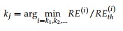 (24)
The synthesis technique described here is implemented using a neural network auto-encoder structure; however, it should be noted that the underlying single-class model can be realized through alternative machine learning paradigms, such as Support Vector Machines (SVM). The selected learning technique must be capable of mapping tightly constrained, compact geographic regions for each target class within the overall feature space.
This section outlines the experimental findings regarding the robustness of various classifiers against adversarial manipulation. The evaluation considers a standard Support Vector Machine (SVM) classifier, an ensemble system configured as a soft voting classifier (VC) [39], and an EnAE classifier constructed via the previously detailed methodology. Implementation of the SVM and VC models was performed using the sklearn library, whereas the EnAE model was developed using the keras framework. These evaluations were conducted using widely recognized benchmark datasets.
To analyze performance, conventional metrics—specifically precision, recall, and F-score—were employed alongside the newly introduced EDCAP metric. The empirical resilience to adversarial manipulation was verified through test instances generated via the protocol outlined in the subsequent subsection.
By conventional definition, an adversarial instance represents a sample from an established class subjected to minimal perturbations, causing a machine learning model to yield an erroneous prediction.
To identify these instances, the approach involves generating a collection of marginally perturbed variants derived from the original training dataset. Any generated instances that provoke an incorrect classification are categorized as adversarial samples for the respective model.
In this investigation, 10 perturbed variants with a feature dimension of N were constructed for every sample in the training set. The perturbation of a given training sample 𝑥∈𝑋𝑇 was achieved by substituting a single feature 𝑥𝑗 with one of 10 uniformly distributed values chosen within the interval from 𝑥𝑗 - 0.05 to 𝑥𝑗 + 0.05. Consequently, each generated test instance varied from its source pattern by only a single feature value. A trial instance was confirmed as an adversarial example if it induced a classification outcome that deviated from the true class of the original sample.
The baseline instance x drawn from the class “3” training data of the Wine dataset [40] and the resulting adversarial instance x∗ produced by altering the initial feature are given below:

The developed model misclassifies the perturbed instance 𝑥∗ as belonging to class “2”. These types of adversarial perturbations are conceptually similar to the one-pixel attacks commonly observed in image classification tasks [20]. Crucially, thousands of such instances typically exist, and the volume of potential adversarial patterns scales upward as the dimensionality of the feature space expands.
This particular framework for producing adversarial data was applied during experiments involving two established benchmarks: Iris [13] and Seeds [14].
This section covers the development and comparative analysis of the SVM, VC, and EnAE models using Fisher’s Iris dataset [13]. This benchmark features three distinct categories across a four-dimensional feature space. The primary dataset was partitioned into an 80% training segment and a 20% testing segment.
To facilitate visualization, the training partition is projected into a two-dimensional framework using the T-SNE dimensionality reduction algorithm (Figure 7).
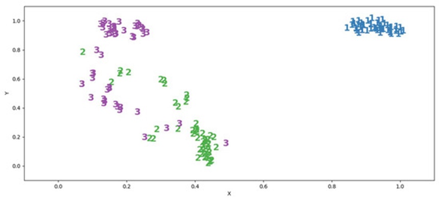
Figure 7. Fisher’s Irises training dataset (different classes colored differently for convenience).
The SVM model was optimized using hyperparameters gamma = 100, C = 10. The VC architecture incorporates a linear support vector machine, a decision tree, and a K-nearest neighbor model. Within the EnAE framework, every constituent auto-encoder utilized the following structural configuration:

The ADAM optimization method was utilized to train all auto-encoders, applying a learning rate of \eta = 0.001. Training for each auto-encoder spanned 3∗105 epochs. The resulting conventional performance metrics computed on the test partition are detailed in Table 5.
Table 5. SVM, VC and EnAE quality assessment by traditional criteria.
Classifier | F-Score | Recall | Precision |
SVM | 0.97 | 0.97 | 0.97 |
VC | 0.97 | 0.97 | 0.97 |
EnAE | 0.98 | 0.97 | 1.00 |
For the derivation of the EDCAP parameters, a scanning resolution step of h = 0.14 was chosen. The resulting EDCAP scores for the models are organized in Table 6.
Table 6. SVM, VC and EnAE quality assessment by EDCAP.
Classifier | Pref | Approx | Coating | Deficit | Excess |
SVM | 1.00 | 0.01 | 1.00 | 0.00 | 93.94 |
VC | 1.00 | 0.01 | 0.66 | 0.33 | 178.9 |
EnAE | 1.00 | 0.08 | 1.00 | 0.00 | 16.82 |
Evaluating the class-specific EDCAP values for the SVM configuration indicated that the complete domain outside the dense regions of categories “1” and “2” is assigned to category “3”. This manner of boundary distribution aligns with the paradigm illustrated in Figure 2b. Conversely, the EDCAP profiles for each class demonstrate that the decision boundaries generated by the VC model more closely reflect the behavior depicted in Figure 2a.
The condition 𝑃𝑟𝑒𝑓=1 denotes that certain categories possess overlapping or ambiguous delineations within the training data. Under these circumstances, a solitary scanning grid cell is simultaneously claimed by the training profiles of two distinct classes. This ambiguity is adjudicated by the models in favor of class “2” for both SVM and VC, whereas the EnAE system favors class “3”.
It is noteworthy that despite achieving excellent results across standard performance indicators, the EDCAP indicators highlight that both the SVM and VC models are inherently more susceptible to adversarial exploits. Furthermore, the 𝑃𝑟𝑒𝑓 metric indicates that the SVM classifier exhibits heightened susceptibility to adversarial manipulation targeted at class “3”.
To verify the actual robustness of these models against adversarial manipulation, 3280 evaluation instances were constructed utilizing the process. Following the categorization of these trial patterns, the frequency of successful adversarial breaches was logged for each specific model and category. The empirical outcomes are compiled in Table 7.
Table 7. Number of successful adversarial attacks against SVM, VC and EnAE.
Classifier | Number of Adversarial Attacks | ||
Class “3” | Class “2” | Class “1” | |
SVM | 115 | 0 | 0 |
VC | 97 | 0 | 0 |
EnAE | 18 | 0 | 0 |
To assist visualization, Figure 8 depicts the training data alongside the successful adversarial exploits targeting the SVM framework within the reduced dimensional space.
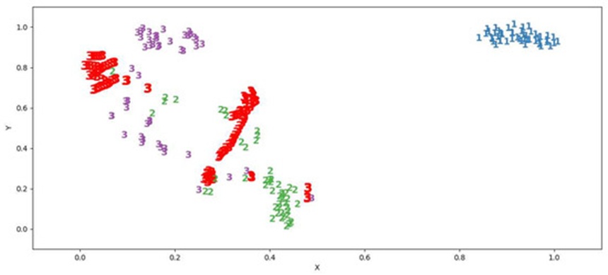
Figure 8. Successful adversarial attacks on the SVM classifier (highlighted in red).
Figure 9 illustrates the successful adversarial breaches accomplished against the VC model.
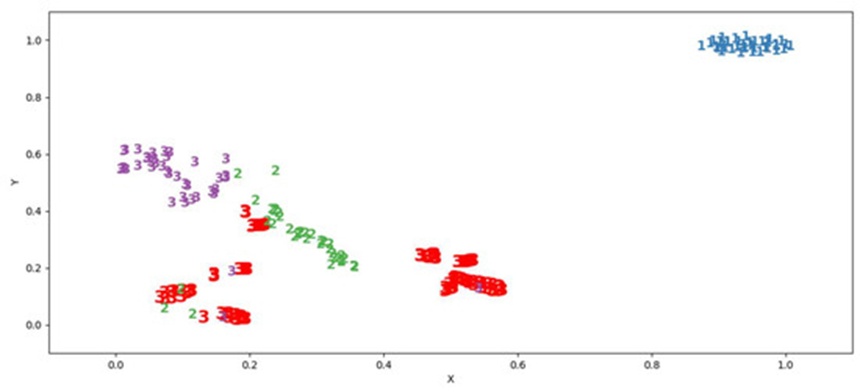
Figure 9. Successful adversarial attacks on the VC classifier (highlighted in red).
Figure 10 displays the training distribution alongside the successful adversarial patterns targeting the EnAE architecture.
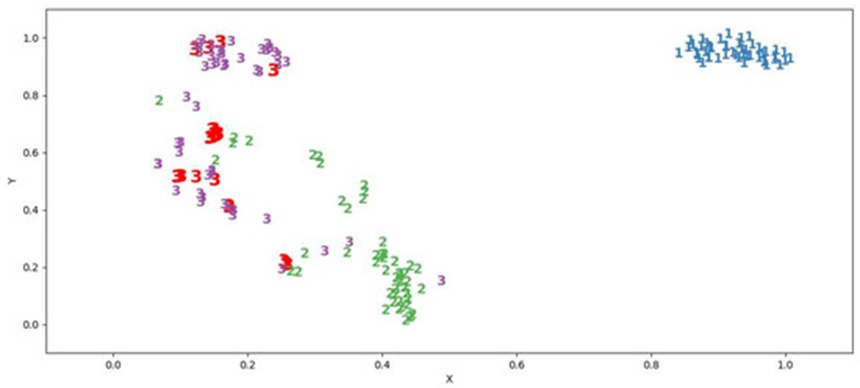
Figure 10. Successful adversarial attacks on the EnAE classifier (highlighted in red).
The resulting empirical robustness profiles of the evaluated models were analyzed through traditional categorization metrics. These performance measures were derived using the collection of modified instances labeled according to their corresponding training source classes. An evaluation was classified as a successful prediction if the model maintained the original label for the perturbed instance. Any shift in classification away from the baseline target indicated an adversarial vulnerability. The performance tracking for the SVM, VC, and EnAE architectures is documented in Table 8.
Table 8. Results of assessing the quality of the classification of adversarial examples.
Classifier | F-Score | Recall | Precision |
SVM | 0.95 | 1.00 | 0.95 |
VC | 0.98 | 0.97 | 1.00 |
EnAE | 0.99 | 1.00 | 0.98 |
The generated experimental evidence confirms that the model developed via the introduced methodology demonstrates superior resilience against adversarial manipulation.
To validate these findings further, the Seeds dataset [14] was selected to replicate the synthesis and comparative evaluation between two model architectures: a Deep Neural Network (DNN) and the EnAE system. This specific dataset comprises three categories represented by 7-dimensional feature vectors. Figure 11 illustrates a two-dimensional mapping of this data generated via the T-SNE technique.
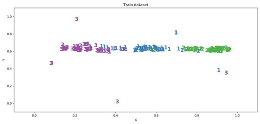
Figure 11. Wheat Seeds training dataset (different classes colored differently for convenience).
For classification purposes on this dataset, a DNN model structured as a multilayer perceptron was implemented, incorporating four fully connected layers, Dropout regularizers, and an output layer utilizing Softmax activation with three output nodes. The architectural layout of the DNN is detailed below:
 (25)
Optimization of the DNN spanned 5∗104 training epochs.
Correspondingly, an EnAE model comprising four neural auto-encoders was constructed for this dataset. The specific internal architecture of each auto-encoder is configured as follows:
The ADAM optimization routine was employed across all auto-encoder networks, configured with a learning rate of 𝜂=0.001 Each individual auto-encoder underwent training for a duration of 3∗105 epochs.
Initially, the performance of both the DNN architecture and the EnAE framework was contrasted utilizing standard classification metrics. The resulting values for precision, recall, and F-score are summarized in Table 9.
Table 9. DNN and EnAE quality assessment by traditional criteria.
Classifier | F-Score | Recall | Precision |
DNN | 1.00 | 1.00 | 1.00 |
EnAE | 0.99 | 0.98 | 1.00 |
Both predictive models display elevated performance levels, with the DNN exhibiting a minor advantage over the EnAE system.
Next, the models were evaluated via the multidimensional EDCAP metric. The EDCAP values provide insight into the expanse of the actual classification decision boundaries relative to the localized training data clusters within the high-dimensional feature space. Within the EDCAP computation routine, the grid spacing parameter for the feature space partition was established at 0.08, yielding a total of 35,831,808 grid cells. The resulting generalized EDCAP assessments for both frameworks are recorded in Table 10.
Table 10. DNN and EnAE quality assessment by EDCAP.
Classifier | Pref | Approx | Coating | Deficit | Excess |
DNN | 0.00 | 0.00 | 0.90 | 0.10 | 735,998.84 |
EnAE | 0.00 | 0.06 | 0.30 | 0.70 | 410.80 |
Analyzing the Excess parameter metrics for both models reveals that the decision domain mapping of the DNN classifier extends far broader outside the immediate training boundaries compared to the EnAE. Consequently, it can be hypothesized that the DNN model possesses greater susceptibility to adversarial exploits than the EnAE framework.
To measure empirical resilience against adversarial attempts using the formulation, 1960 perturbed evaluation instances were constructed. Following the processing of these instances through the models, the frequency of successful adversarial disruptions was quantified. These experimental findings are provided in Table 11.
Table 11. Number of successful adversarial attacks on classifiers.
Classifier | Number of Adversarial Attacks |
DNN | 759 |
EnAE | 43 |
The documented metrics indicate that the DNN architecture suffered over 17 times more successful adversarial breaches than the EnAE system. For visual clarity, Figure 12 illustrates the training observations along with successful adversarial attacks impacting the DNN model, while Figure 13 shows the corresponding patterns for the EnAE classifier. Class labels yielding predictions inconsistent with neighboring training observations are highlighted in red.
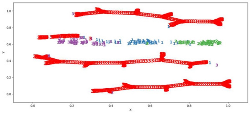
Figure 12. Successful adversarial attacks on the DNN classifier (highlighted in red).
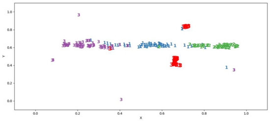
Figure 13. Successful adversarial attacks on the EnAE classifier (highlighted in red).
Correlating the empirical test outcomes with the derived EDCAP metrics substantiates the core hypothesis that the EnAE classifier possesses superior robustness against adversarial perturbations. Additionally, these findings underscore that the multidimensional EDCAP methodology offers a means to measure classification performance not only within the training distribution space but also throughout external regions.
To gauge the utility of the introduced design methodology, the categorization performance on adversarial patterns was audited using conventional metrics. These indicators were computed across the set of perturbed patterns utilizing labels inherited from the baseline training distribution. The resulting evaluation statistics for both the DNN and EnAE setups are compiled in Table 12.
Table 12. Results of assessing the quality of the classification of adversarial examples.
Classifier | F-Score | Recall | Precision |
DNN | 0.61 | 0.61 | 1.00 |
EnAE | 0.99 | 0.98 | 1.00 |
The established traditional performance indicators verify that the DNN model exhibits a pronounced vulnerability to adversarial manipulation relative to the ensemble of auto-encoders (EnAE) developed under the proposed framework.
Collectively, these empirical outcomes validate the utility of EDCAP tracking to reliably measure the adversarial resilience of machine learning classifiers.
The primary contributions of this study encompass:
A novel methodology for evaluating the behavioral attributes of classifiers beyond the bounds of the training data;
An investigation into and determination of the underlying triggers for machine learning classification failures, including those induced by adversarial manipulation;
The introduction of the multidimensional EDCAP metric designed to quantify the performance of multiclass classification systems;
A new EnAE classification framework utilizing an ensemble of auto-encoders, engineered to exhibit superior resilience against adversarial manipulation compared to conventional artificial neural networks, SVMs, and related frameworks.
The core significance of this research lies in its explanation of why classification errors manifest and why adversarial interventions succeed. The introduced strategy for minimizing classification discrepancies relies on managing the spatial boundaries a model establishes following its training phase. Consequently, new assessment metrics for evaluating both single-class and multiclass classification architectures are formulated.
The proposed multidimensional EDCAP metric provides a standardized means to contrast diverse models based on their respective levels of adversarial resilience. This assessment tool is universally applicable, remaining completely decoupled from the underlying model architecture or the specific protocol used to construct adversarial instances.
Empirical testing confirms that the developed synthesis pipeline and the corresponding EnAE multiclass classification routine yield higher resistance to adversarial exploits than SVMs, ensemble paradigms, and deep neural networks. This robust behavior can be directly interpreted through the provided conceptualization of adversarial mechanics alongside the inherent geometric properties of auto-encoders.
It should be emphasized that within this synthesis pipeline, alternative single-class classification models—such as one-class SVMs—can be integrated into the ensemble structure in place of auto-encoders. The essential requirement is that the combined ensemble correctly implements the necessary decision logic and training optimization mechanisms.
The distinct benefits and drawbacks of these methodologies warrant closer examination. The principal operational traits of the introduced multidimensional metrics for measuring adversarial resilience include the following:
They facilitate the pre-deployment assessment of a model's susceptibility to adversarial manipulation and systemic failures;
They are compatible with any classification architecture;
They function effectively within high-dimensional feature spaces where traditional visual inspection is impractical;
The multiclass model assessment accounts for overlapping class boundaries and documents the model's preferred classifications within those shared zones;
They provide an objective framework for characterizing classification performance outside the training data distribution, offering numerical estimates of decision space stability in high-dimensional settings.
Conversely, the multidimensional EDCAP metric exhibits the following limitations:
Marked sensitivity regarding the selected dimensions of the feature space discretization grid cells;
Substantial memory overhead requirements when conducting operations in high-dimensional settings;
A polynomial computational complexity where the polynomial degree scales with the dimensionality of the feature space, hindering direct deployment in high-dimensional tasks such as image analysis.
Despite these computational constraints, alternative strategies for diagnosing model behavior outside the training dataset were not identified in existing literature. Furthermore, the EDCAP computation pipeline remains amenable to optimization through refined algorithmic design and specialized hardware acceleration (GPGPU).
Determining the ideal grid cell resolution for partitioning the active feature space during classification remains a highly critical, unresolved challenge. The specific heuristic guidelines adopted in this study require deeper analysis.
On one hand, choosing an excessively large grid resolution minimizes the computational overhead. On the other hand, it diminishes the precision of the resulting EDCAP values, rendering them ineffective. Conversely, overly reducing the grid step is also counterproductive due to the exponential rise in EDCAP processing requirements. Moreover, past a certain threshold of granularity, a significant portion of the grid cells situated within the training data domain become vacant, which undermines the reliability of the calculated EDCAP metrics. Consequently, an optimal resolution threshold must exist, which can be defined by a basic heuristic rule: within the bounded training domain of a given class, every discrete cell must encompass at least one training observation. Future inquiries may yield a systematic framework for deriving this optimal step size for any given dataset.
The introduced approach for building resilient EnAE models is distinguished by the following characteristics:
It supports the synthesis of classifiers with controllable levels of resistance to adversarial interference and processing errors;
The mechanisms underlying its adversarial defenses are mathematically justified by the reconstruction properties of the underlying auto-encoders;
Model optimization can be advanced by tuning the auto-encoder configurations to match the specific profiles of individual classes;
It accommodates auto-encoders constructed via either support vector machines or neural network architectures.
However, the EnAE synthesis paradigm is subject to the following constraints:
The model's ultimate adversarial resilience is highly dependent upon both the initial weight distributions and the chosen structural configuration of the auto-encoder neural networks;
For applications featuring an exceptionally high number of target classes, training a separate one-class model for every individual category demands extensive computational resources.
Deploying this synthesis framework will enable practitioners to regulate classification error rates and foster greater confidence in machine learning pipelines. Elevating the reliability of these machine learning frameworks will subsequently expand their viability across real-world operations.
This study investigated the systemic errors characteristic of machine learning classifiers and explained the mechanics driving successful adversarial exploits against them. A new multidimensional assessment metric (EDCAP) was introduced to evaluate the robustness of multiclass models against adversarial interference. Additionally, the EnAE classification routine—predicated on an ensemble of neural network auto-encoders—was developed alongside its corresponding synthesis framework. The EnAE approach operates by constructing constrained, dense decision zones for separate classes within the feature space, utilizing a hard voting decision strategy. This structural feature empowers the system to distinguish recognized classes from anomalous or external samples lying outside the core training data distribution. Furthermore, this design allows for the detection of out-of-distribution inputs located far from the training clusters. The multidimensional EDCAP metric enables developers to evaluate how closely an active decision boundary aligns with original training observations, allowing for targeted model tuning to achieve the desired level of adversarial protection. The synthesis of two distinct EnAE classifiers using publicly accessible, multidimensional datasets was demonstrated and compared against traditional architectures, including SVMs, soft voting classifiers, and deep neural networks. The empirical results confirm the superior performance of the proposed EnAE classification framework relative to traditional methodologies. Finally, the defining attributes, advantages, and limitations of these approaches were detailed, establishing a roadmap for future investigations aimed at broadening the practical utility of these findings.
None
None
The reported study was funded by RFBR according to the research project No. 20-37-90073.
None
Open Access The author(s) retain copyright. This article is licensed under the Creative Commons Attribution-NonCommercial-ShareAlike 4.0 International License. It may be shared and adapted for non-commercial purposes with appropriate attribution, an indication of changes, and distribution of adaptations under the same license. Third-party material may be subject to separate terms identified in its credit line. View the license at https://creativecommons.org/licenses/by-nc-sa/4.0/.
 Transparent Intelligence Publishing