Recently, significant efforts have been dedicated to enhancing anomaly detection methods, especially concerning high-dimensional and distributed clinical datasets. The analysis of patient information in clinical environments highlights a strong emphasis on improving diagnostic precision, tailoring treatment strategies, and maximizing resource efficiency to boost health outcomes. However, this field encounters distinct difficulties, including sporadic data gathering, variable data quality, and structural differences unique to individual patients. To overcome these obstacles, this paper introduces an innovative hybrid framework that merges stochastic and heuristic techniques for detecting anomalies in clinical patient data. This approach leverages an HPO-optimized Density-Based Spatial Clustering of Applications with Noise to group patient exercise data, thereby streamlining the detection of abnormalities. Following this, an Interquartile Range-based stochastic technique filters out untrustworthy data points, guaranteeing that healthcare practitioners and diagnostic systems are supplied with only highly relevant and precise data. The main goal of this research is to provide medical experts and scholars with a reliable instrument for handling vast, high-dimensional clinical datasets, allowing for the successful separation and elimination of deviant data observations. Additionally, an advanced regression model was constructed utilizing Automated Machine Learning (AutoML) to evaluate the effectiveness of the ensemble technique for detecting abnormal patterns. Multiple statistical error evaluation methods are employed to verify the success of this hybrid strategy in conjunction with AutoML. Empirical findings indicate that applying this cutting-edge hybrid framework to patient rehabilitation data significantly boosts AutoML performance, yielding an average improvement of 0.041 in the score, thereby outperforming conventional regression models.
In recent times, data volumes have expanded exponentially across multiple domains of everyday life, such as healthcare [1], finance [2], and smart manufacturing [3]. Within the healthcare sector, data generation has escalated from 500 petabytes in 2012 to 25,000 petabytes by 2022 [4]. Nevertheless, immense quantities of healthcare data harbor anomalies, uncertainties, and contradictions due to their highly dimensional and distributed nature. Consequently, addressing irregular data patterns to assist medical professionals by extracting actionable insights continues to be a critical and expansive area of study within data mining (DM) [5, 6]. Investigators must be capable of identifying aberrant data to acquire the foundational knowledge required for improved decision-making in data analysis. The challenges introduced by massive, multidimensional datasets are substantial, given that such collections invariably include some degree of anomalous information, irrespective of their overall scale [7]. Spotting these anomalies represents a formidable hurdle in DM due to the scarcity of labelled data representing unconventional cases. As a result, numerous techniques employed for identifying anomalies operate in a fundamentally unsupervised manner [8]. A primary example of this is pinpointing observations that diverge significantly from the remainder of the dataset. Still, formulating a universally applicable mathematical definition for deviation continues to be an unachieved goal across diverse datasets and contexts.
The unsupervised character of anomaly detection frequently results in a significant gap between instances that are statistically rare and those that hold true clinical relevance, particularly within healthcare environments. This difficulty is further exacerbated by the escalating complexity and sheer size of datasets, which are propelled by technological progress in medical devices, computing hardware, and related fields. Conventional approaches, including ensembling, sub-sampling [9, 10], deep learning [11], and density peak clustering [12], are routinely modified to manage the widespread distribution and high-dimensional nature of this data. Despite this, isolating significant irregularities remains a complex task, driving the need for anomaly detection frameworks that are more precise, adaptable, and highly efficient.
Additionally, the significance of an anomaly can fluctuate depending on its context, heavily impacted by variables like seasonal shifts and precise temporal units [13]. For example, an elevated heart rate that seems unusual might actually be anticipated following physical exertion, much like variations seen in seasonal product sales or power consumption trends. Contemporary anomaly detection systems need to accommodate these fluctuations by utilizing specialized tools to distinguish between genuine abnormalities and deviations that are contextually justifiable [14, 15]. Current studies aim to improve these methodologies, ensuring that the detection of anomalies in clinical records does not cause the deletion of crucial data, a mistake that could trigger severe consequences for patient care [16, 17]. This underscores the urgent requirement for ongoing advancement in anomaly detection strategies that are attuned to the subtleties of clinical information while remaining resilient against false positive results.
Explainable anomaly detection has grown in popularity, leveraging advanced models such as copulas to improve interpretability. For example, the COPOD framework, detailed in a prior study [18], creatively calculates tail probabilities via empirical copulas, thereby refining the accuracy of anomaly identification in medical settings. Furthermore, the detection of multivariate anomalies has been investigated using diverse approaches, including clinical trial-driven systems [19] and rigorous statistical methods. The Hawkins dataset, for instance, acts as a foundational benchmark in multiple investigations, such as the research conducted by Gao et al. [20], which contrasts the Max-Eigen Difference method with conventional Robust and Mahalanobis distance metrics for identifying multivariate anomalies. Additional advancements encompass the revelation of multivariate anomalies via original methodologies, as analyzed by Southworth [21], alongside the implementation of non-parametric multivariate depth functions to consistently differentiate between typical and aberrant data [22]. Together, these approaches highlight the persistent endeavors to optimize anomaly detection pipelines, rendering them more practical and interpretable within medical environments.
Current techniques possess multiple drawbacks, primarily because the majority are explicitly structured to tackle anomalous instances using supervised datasets. These strategies, however, require massive quantities of training data, the collection and analysis of which are highly resource-intensive. Consequently, the efficacy of these approaches falls short when managing anomalous data points in critical sectors like healthcare. Additionally, the curse of dimensionality restricts the capacity of these methods to discover patterns within low-dimensional data. The success of these techniques in proving the necessity and reliability of managing abnormal data trends within the healthcare sector remains unverified. Thus, a robust and reliable methodology for detecting abnormal patterns is required to process clinical patient data, ensuring that anomalies are identified while equipping medical practitioners with only the most relevant patient details. To effectively recognize anomalous observations within vast clinical datasets, this research introduces a hybrid anomaly detection system that merges stochastic and heuristic approaches. Furthermore, the key contributions of the presented hybrid framework are outlined as follows:
Developing an advanced data preprocessing module capable of executing diverse operations to improve the precision and quality of the acquired patient records.
Formulating a hybrid anomaly detection strategy that integrates heuristic and stochastic methodologies to pinpoint irregular data behaviors in patient datasets, thereby empowering healthcare professionals to care for patients by providing only relevant information exclusively.
Evaluating the capability of the designed hybrid anomaly detection framework to isolate strange data behavior in clinical data by employing the Automated Machine Learning (AutoML) paradigm.
Integrating various statistical evaluation methods to validate the performance and underscore the significance of the proposed research investigation.
Anomaly detection, which involves recognizing departures from normal behavior, is vital in machine learning (ML) and the evaluation of medical data, especially for enhancing the precision and dependability of forecasting models. This segment structures the relevant literature into three primary classifications: Anomaly Detection in ML, Anomaly Detection in Medical and Clinical Applications, and Statistical and Computational Techniques for Anomaly Detection.
Within the domain of ML, anomalies are generally viewed as infrequent incidents or data points that stray from typical trends, requiring further examination because of their irregularity. Common instances involve unexpected shifts in activity levels, textual mistakes, or rapid fluctuations in temperature [23-25]. In this setting, both ML and data mining (DM) strategies have advanced to tackle anomaly detection through algorithms like Decision Trees, Naive Bayes, and Bayesian Networks, all of which are highly regarded for being straightforward and efficient [26]. As an illustration, the K-Nearest Neighbour technique is widely used due to its strong performance in proximity-driven learning, even though it demands significant storage and computational power [27].
Additional progress in anomaly detection using ML focuses on differentiating actual problems from erroneous alerts. Zheng et al. [28] created a training dataset aimed at pinpointing vulnerabilities, which aids in eliminating false positives during static analysis and enables developers to effectively prioritize real security threats. The scope of anomaly detection has also broadened to include Autoencoders and Generative Adversarial Networks (GANs) within medical contexts, including their use in optical coherence tomography to find abnormalities [29] and in detecting early-phase kidney transplant rejections [30]. Nevertheless, major hurdles persist, most notably elevated false-positive frequencies and the necessity for uniform standards regarding what classifies as an anomaly [31-33]. Such limitations highlight the critical need to improve ML algorithms to decrease computational demands and boost their real-world utility.
Identifying anomalies is fundamental to the evaluation of clinical and medical data, as the prompt recognition of irregular trends can facilitate early interventions and yield better patient health outcomes. Techniques utilizing minimum spanning trees, proposed by Li et al. [34, 35], manage outliers within intricate medical databases, thereby improving diagnostic precision. Additionally, Gijzel et al. [36] offered perspectives on forecasting physical robustness and resilience using diverse assessments, although additional research is necessary to overcome barriers to clinical application.
Comprehensive meta-analyses, like the study conducted by Ji et al. [37], emphasize that data-centric approaches can lower the relative risk associated with cardiac incidents. Nonetheless, these results might not be broadly applicable to every demographic. Gevaert et al. [38] suggested tailored physical activity programs that account for personal variations, including genetic predispositions. Conversely, Morris et al. [39] observed that rehabilitation programs centered around exercise enhanced the living standards of individuals suffering from pulmonary hypertension. In a related vein, Babaei et al. [40] investigated wearable accelerometers in the context of physical therapy, Dibben et al. [41] evaluated cardiac recovery strategies for coronary heart disease, while Cheng et al. [42] and Gu et al. [43] performed meta-analytic studies focusing on pulmonary rehabilitation (PR) among patients diagnosed with interstitial lung disease.
A multitude of investigations back the effectiveness of PR in mitigating shortness of breath and boosting exercise tolerance in individuals with long-term respiratory ailments, as seen in [44-47]. As another illustration, Rasheed et al. [48] investigated ML algorithms for forecasting seizures early using electroencephalogram readings, whereas Li et al. [49] analyzed multiple ML frameworks for categorizing cardiovascular conditions. Additional medical applications for anomaly detection encompass monitoring patient body positions via long short-term memory (LSTM) architectures [50] and deploying data fusion strategies to mitigate data sparsity, as demonstrated by Yang et al. [51]. Furthermore, Zhang et al. [52] showcased the capability of convolutional neural networks (CNNs) in handling the binary classification of skewed datasets. Finally, Liu et al. [53] and Zhao et al. [54] utilized ML systems to analyze rehabilitation metrics and patient records, respectively.
Due to their straightforwardness and efficiency, statistical approaches serve as a cornerstone in the field of anomaly detection. One prevalent technique is thresholding, which uses predetermined boundaries to flag anomalies; this was illustrated by Amores et al. [55], who utilized a smart waste receptacle equipped with gas detectors to track food freshness. Analysis of Variance, another conventional approach, assesses meaningful disparities among categories and proves highly useful for spotting atypical data patterns [56].
Advanced architectures, like Expectation-Maximisation ensemble unsupervised clustering guided by supervised techniques, are specifically designed for grouping tasks. These have shown enhanced precision in evaluating psychiatric disorders, outperforming alternative methods by roughly +1.9 points [57]. To improve dependability, Li et al. [58] introduced the Poincare distance measurement for spotting anomalies within electronic health records. Meanwhile, Amanullah et al. [59] emphasized the predictive value of extra-aortic valvular heart irregularities in individuals with aortic stenosis, correlating condition severity with negative clinical events and mortality. Furthermore, Peng et al. [60] applied a latent correlation approach to analyze anxiety and mood disorders; although they faced difficulties in forming a common latent framework, their work highlighted the necessity for specialized analytical methods in psychopathology.
Ultimately, statistical methodologies are integral to the examination of rehabilitation data. Frameworks such as LSTM and CNN assist in tracking the recovery progress of patients [50, 52], whereas risk evaluation models offer crucial instruments for predicting clinical outcomes [56]. While these investigations emphasize the flexibility of computational and statistical methods in identifying anomalies, challenges related to their scalability and capacity to process high-dimensional datasets remain.
This segment details the methodology recommended in this paper. Pinpointing anomalies within patient rehabilitation data requires a highly responsive and dependable system capable of finding irregular observations while delivering improved predictive capabilities. The medical sector presently faces complex hurdles introduced by advanced technologies, which complicates the identification of aberrant data. Because these decisions carry potential life-threatening consequences, accuracy in this field is paramount.
Atypical data trends represent irregular behavior within a data stream that deviates from the expected norm. Utilizing both stochastic and heuristic strategies is essential for recognizing and handling these deviations. This research leverages Hyperparameter Optimisation (HPO-based) tuned Density-Based Spatial Clustering of Applications with Noise (DBSCAN) as its heuristic mechanism to detect and isolate irregular data sequences, thereby strengthening overall data integrity. Concurrently, stochastic approaches incorporate statistical functions—such as level shift, range, thresholding, and mean—to accurately locate aberrant data points. To achieve greater accuracy, this research implements a combined strategy that merges stochastic and heuristic models for superior anomaly detection. Figure 1 illustrates the proposed architecture for managing anomalous data.
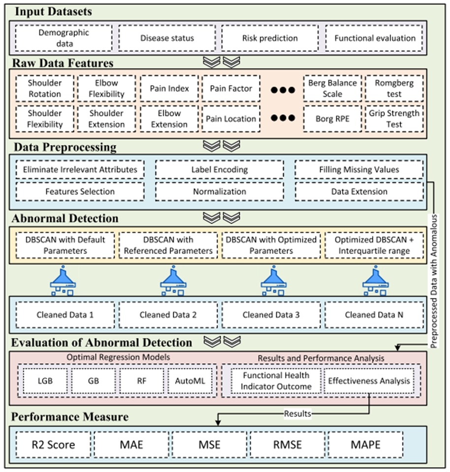
Figure 1. Recommended hybrid model for anomaly detection. AutoML, automated machine learning; DBSCAN, density-based spatial clustering of applications with noise; LGB, light GB; MAE, mean absolute error; MAPE, mean absolute percentage error; MSE, mean squared error; RF, random forest; RMSE, root mean squared error.
A major hurdle in managing anomalies is the scarcity of data across all sectors, particularly in healthcare. Regrettably, to validate our proposed framework, the original dataset contains a limited number of instances characterized by high unreliability and missing entries. Therefore, the acquired data initially undergoes a preprocessing phase to address these inconsistencies, transforming it into a viable format for subsequent predictive modelling.
To improve data uniformity and quality, an adaptive imputation approach is utilized to populate missing entries. This research applies zero-based and K-nearest neighbors imputation methods for continuous variables, whereas predictive analytics is deployed to resolve missing categorical data. Following preprocessing, the dataset remains too sparse for the effective training of deep learning architectures. Consequently, it is necessary to expand this restricted dataset into a robust synthetic collection to guarantee accurate model optimization. To accomplish this, the GAN augmentation method is implemented, producing synthetic instances from the original data to comprehensively train the algorithms.
The central aim of this investigation is to forecast anomalous instances within clinical records to facilitate successful patient rehabilitation. To evaluate the impact of removing these abnormalities, baseline experiments are executed on the pristine augmented dataset, recording the baseline performance of each algorithm. Following this, the DBSCAN algorithm is executed on each dataset using the configurations specified in this research [61] to assess predictive model efficacy. To ensure optimal anomaly detection, HPO is deployed to fine-tune the DBSCAN parameters for each specific dataset. To purge irregular data structures from the augmented dataset, a sophisticated hybrid anomaly detection framework is introduced, merging Stochastic and Heuristic methodologies. This integrated model combines an IQR-enhanced stochastic approach with optimized DBSCAN to isolate and discard anomalous entries across the four datasets. Post-removal, the reliability of the clinical data is re-evaluated using the same models. The comparative predictive outcomes are subsequently illustrated in Figure 2, measuring the model's effectiveness in filtering aberrant patterns from the dataset.
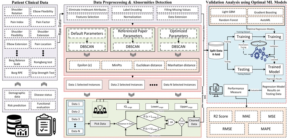
Figure 2. Proposed design schematic for identifying anomalies in clinical data. DBSCAN, density-based spatial clustering of applications with noise; IQ, interquartile; MAE, mean absolute error; MAPE, mean absolute percentage error; MSE, mean squared error; RMSE, root mean squared error.
The IQR serves as a statistical metric to pinpoint outliers within a given dataset. To compute the IQR, the observations are initially ordered and partitioned into three quartiles: the first quartile (Q1), the median (Q2), and the third quartile (Q3). The IQR represents the spread between Q3 and Q1, capturing the central 50% of the distribution. Outlier detection boundaries are established at Q1 − 1.5IQR for the lower limit and Q3 + 1.5IQR for the upper limit. Observations falling beyond these thresholds are classified as outliers or anomalies, as depicted in Figure 3. This mathematical strategy is particularly advantageous for datasets exhibiting skewed or non-normal distributions, as it isolates the dispersion of the central 50% of the values, successfully eliminating extreme outliers that might skew statistical evaluations.
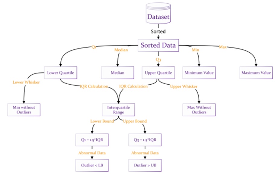
Figure 3. Working of interquartile range abnormal detection.
Anomaly detection methodologies primarily concentrate on recognizing variations from typical behavioral norms. The objective is to define a standard of normal activity and delineate a corresponding acceptable operational zone. To accomplish this, an algorithmic procedure is designed to separate standard data from anomalous instances, as illustrated in Algorithm 1. The recommended hybrid methodology for pinpointing irregular observations encompasses several progressive stages.
Initially, the amassed dataset undergoes a purification procedure, eliminating static and redundant variables to minimize processing overhead. Subsequently, a hybrid technique merging the k-NN algorithm with predictive analytics is deployed to resolve missing feature values. The refined dataset is then evaluated using the DBSCAN algorithm to spot preliminary outliers in the patients' exercise and clinical records. This initial execution of DBSCAN utilizes the parameters detailed in Ref. [61], with findings documented according to these predetermined configurations.
Additionally, the HPO technique is employed to optimize the hyperparameters for each distinct dataset, guaranteeing the DBSCAN algorithm operates at peak efficiency. Following this optimization, DBSCAN is coupled with an IQR-driven stochastic method to identify observations that diverge from standard patterns within every dataset. This IQR-based stochastic mechanism operates through consecutive steps: first, the inter-quartile range of the dataset is calculated. This metric is then multiplied by a constant coefficient of 1.5. The resulting product is added to the third quartile; any data point surpassing this total is flagged as anomalous. In parallel, this same product is subtracted from the first quartile, and observations falling beneath this threshold are similarly categorized as anomalous. Together, these procedures facilitate the accurate detection of potential outliers within the data.
This systematic framework effectively separates and removes anomalous (outlier) observations from the prepared data, providing healthcare practitioners with essential diagnostic insights to subsequently monitor patient rehabilitation.
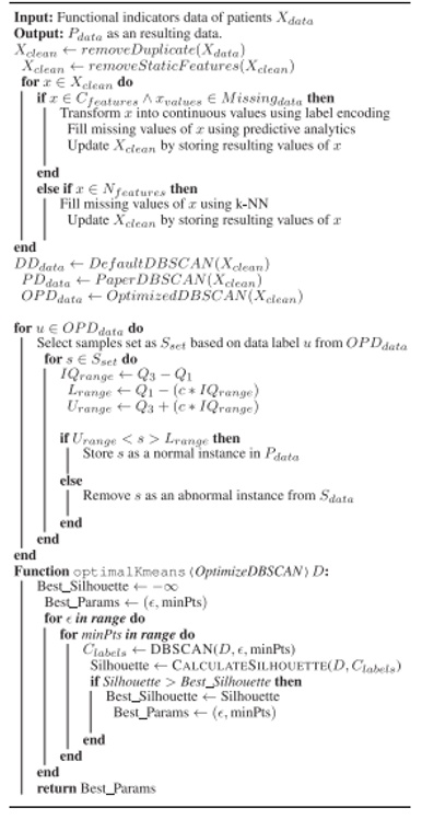
Algorithm 1. Hybrid approach for identifying atypical data points within clinical and exercise-related patient data.
Algorithm 2 outlines a comprehensive methodology for assessing the performance of the newly designed anomaly detection framework, emphasizing the application of AutoML. This algorithm operates through several pivotal phases:
The procedure commences by elevating data integrity via preprocessing, as detailed in Algorithm 1. Following this preparation, the data is split into training (identified as Strain) and testing (identified as Stest) partitions. Subsequently, AutoML is employed to refine the model training phase, particularly for a dedicated regression objective. The increasing popularity of AutoML stems from its capability to autonomously construct ML frameworks, rendering it a vital asset. The next step entails identifying the most proficient regression algorithm based on the training outcomes generated by AutoML. This selected algorithm is then applied to measure the success of the hybrid framework in forecasting health-centric parameters.

Algorithm 2. A refined regression methodology using AutoML is employed to assess the efficacy of the suggested hybrid model in detecting anomalies.
By automating the evaluation and tuning of ML frameworks, AutoML significantly streamlines the entire pipeline. This optimized methodology boosts operational efficiency and conserves substantial computational and temporal resources that would otherwise be expended on manual tuning. Moving to the fifth step, the efficacy of the AutoML-selected framework is analyzed utilizing the testing samples. Crucial evaluation metrics—including Mean Absolute Error (MAE), Mean Squared Error (MSE), Root Mean Squared Error (RMSE), Coefficient of Determination (Rscore), Root Mean Squared Logarithmic Error (RMSLE), and Mean Absolute Percentage Error (MAPE)—are applied to assess prediction precision, providing critical insights into the framework's testing performance. Ultimately, the final phase contrasts the optimized AutoML regression framework against several baseline algorithms, namely XGBoost (XGB), Light GB (LGB), and Random Forest (RF). This comparative analysis is vital for validating the overall effectiveness of the hybrid methodology in isolating anomalies within the designated clinical datasets.
To validate the performance of the proposed hybrid framework, authentic clinical data was acquired from Jeju National University (JNU) located in South Korea. This investigation focuses on the medical logs of individuals undergoing rehabilitation for Adhesive Articular Cystitis. The gathered dataset incorporates critical parameters, including patient demographics, pathology details, risk evaluations, and functional capacity metrics. The demographic segment encapsulates fundamental personal details like ID, name, and gender. The pathology status is comprehensively documented with variables such as contemporary health status, physical activity levels, specific rehabilitation routines, disease categorization, primary symptoms, symptom onset dates, and appointment schedules. The risk prediction category involves diverse elements encompassing both medical and personal histories. For the functional capacity assessment, the data features clinical measurements such as grip strength (right and left), arm curl tests (right and left), and the Push-up test. Within this specific database, conventional attribute names are replaced; instead, each variable is designated a unique ‘data code’. The application of this genuine patient information is fundamental to corroborating the reliability of the suggested hybrid framework in anomaly detection.
Data preparation is dedicated to purifying and reformatting information into a stable structure to facilitate the extraction of underlying trends and insights. This preparatory stage encompasses several distinct operations designed to yield dependable, high-fidelity data. These procedures involve identifying and discarding duplicate entries within the database. Moreover, static and irrelevant attributes are removed to lessen storage requirements and computational strain. Multi-valued features are refined to guarantee that each parameter preserves atomicity. To resolve missing entries, a hybrid imputation methodology combining k-NN and predictive methods is implemented. Transformation protocols are applied to convert data values into machine-readable formats. Finally, normalization techniques are deployed to scale values within a predefined spectrum, ensuring consistency across all attribute measurements.
Figure 4 illustrates the results of a Pearson correlation assessment conducted on the functional capacity variables. This analytical method determines the linear association between a given pair of attributes utilizing the Pearson correlation coefficient, which ranges from −1 to 1. A score of 1 indicates a flawless positive linear relationship, whereas −1 signifies a flawless negative linear relationship, and a score of 0 denotes the absence of any linear correlation between the variables. Pearson's r is extensively applied in statistical analysis to quantify the strength of linear dependencies between different variables.
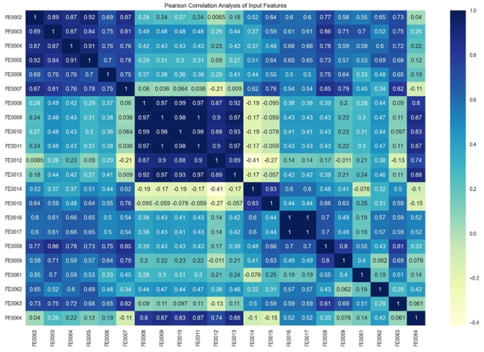
Figure 4. Identifying key features through the application of correlation analysis.
The correlational matrix depicted in Figure 4 serves as a structured table illustrating the correlation coefficients between various sets of variables. It is crucial to note that the diagonal coordinates of this matrix uniformly display a value of 1, denoting that every variable perfectly correlates with itself.
Through the application of correlation analysis, attributes within the dataset that display positive and negative associations are identified. For this experimental framework, attention is strictly directed toward positively correlated attributes, while those exhibiting negative correlations are intentionally excluded from the dataset. As illustrated in Figure 4, only a trio of features—FE0015, FE0014, and FE0007—display a negative correlation with the target variables within this specific dataset. This calculated exclusion ensures the analysis concentrates exclusively on features that favorably align with the targeted outcomes for further investigation.
Machine learning (ML) frameworks, particularly deep learning models, necessitate a rigorous training regimen dependent on extensively annotated datasets. Nevertheless, the acquisition, retention, and preparation of such comprehensive datasets can be prohibitively costly. Furthermore, the efficacy of these models relies on the availability of a substantial volume of high-quality, labeled training records, often reaching tens of thousands or more. Consequently, there is an urgent requirement for a methodology to expand limited datasets into more substantial synthetic versions, thereby facilitating the creation of generalized models.
This research proposes an innovative technique titled the GAN-assisted Time GAN augmentation method. This approach broadens restricted datasets into larger collections by generating synthetic samples based on original data. Additionally,
Figure 5 provides a visual representation of the impact of data augmentation using GANs, illustrating the increase in data volume before and after the process. Initially, the instance count for each dataset is approximately one thousand; post-augmentation, this count is elevated to ten thousand for each set. This expansion significantly boosts the size of the dataset, contributing to more efficient and generalized model training.
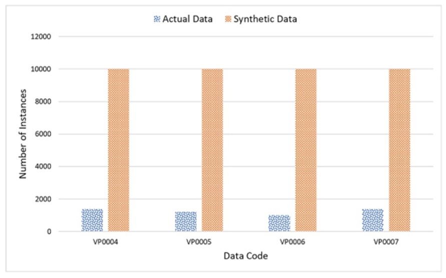
Figure 5. Actual and synthetic data for the experiments.
Table 1 outlines the diverse software and technological infrastructure utilized to construct the proposed data and predictive analytics architecture. Python serves as the primary programming language for the experiments in this study. Various essential Python packages, including Sklearn, ydata_synthetic, ctgan, Pycaret, and ADTK, were employed. Additionally, Microsoft Excel was utilized for the storage of both raw and processed datasets.
Table 1. Tools and technologies used in experimentation.
System Component | Specifications / Details |
Operating System | Windows 11 OS |
Main Memory | 96 GB RAM |
Processor (CPU) | Intel Core i9-12900K (12th Gen) @ 3.20 GHz |
Programming Language | Python 3 |
Development IDE | PyCharm Professional Edition |
Database | MS Excel, MySQL |
Key Toolkits / Libraries | Pandas, Scikit-learn, Seaborn, Matplotlib, ydata-synthetic, CTGAN, AutoML, DBSCAN, etc. |
Abbreviation: IDE, integrated development environment.
This section describes the findings of employing DBSCAN for anomaly detection across four distinct datasets: the Borg rating of perceived exertion (RPE), the TUG, the Romberg Test, and the Berg Balance Scale (BBS). We utilize a structured methodology encompassing preliminary visualization, the application of parameters established by Braei and Wagner [61], parameter refinement via grid search, and a hybrid strategy merging DBSCAN (with optimized parameters) and the IQR for improved abnormality identification. A fundamental operational guide for DBSCAN is provided in Algorithm 3, detailing the core procedures of the algorithm. Algorithm 3 requires three primary parameters:
Data: The dataset currently under analysis.
ε (Epsilon): The radius utilized by the algorithm to locate neighboring data points for each observation.
Minimum Points (MinPts): The required number of observations within the ε -vicinity of a specific point to designate it as a core point.
The procedural flow is as follows:
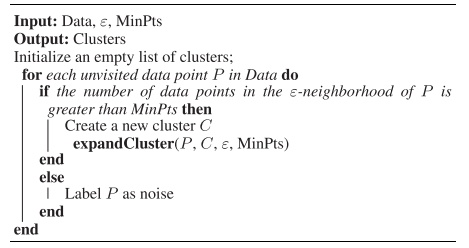
Algorithm 3. DBSCAN algorithm
The algorithm traverses each unvisited data point. For every point, it checks whether the count of data points within the ε -neighborhood exceeds the MinPts threshold.
If the condition is satisfied, a new cluster is initialized, and the expandCluster function is invoked to expand the cluster by recursively incorporating connected points. If the condition is not satisfied, the point is classified as noise.
In the DBSCAN algorithm, the ε -neighborhood Nε (P) of a point P is defined as the collection of all points q where the distance from P is less than or equal to ε, as expressed in Eq. 1:
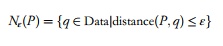 (1)
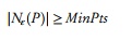
A point P is identified as a core point if the number of points within its ε -neighborhood is greater than or equal to the minimum point threshold MinPts, as expressed in Eq. 2:
 (2)
We begin by acquiring insights into the datasets through basic visualization techniques, as illustrated in Figure 6. This visualization clarifies the inherent structure of the data and provides a foundation for selecting appropriate parameters for the DBSCAN algorithm.
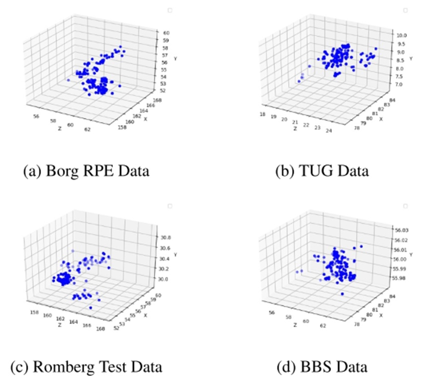
Figure 6. A simple visualisation of four data before abnormal detection. BBS, Berg Balance Scale.
Subsequently, we implement DBSCAN on the datasets utilizing parameters sourced from the referenced study [61]. The DBSCAN algorithm functions by identifying dense regions in the data, categorizing points with insufficient density as noise. It assigns labels based on connectivity and density using the parameters defined in the reference [61]. A visual depiction of abnormal detection in four datasets using DBSCAN with reference paper parameters is presented in Figure 7.
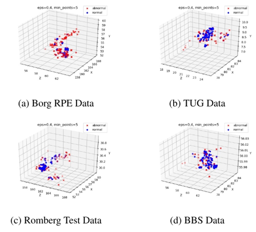
Figure 7. Visualisation of abnormal detection of density-based spatial clustering of applications with noise with reference paper parameters. BBS, Berg Balance Scale.
To improve the performance of DBSCAN, we execute parameter optimization via grid search. We investigate a range of ε and MinPts values to determine the optimal combination that best aligns with the specific characteristics of each dataset. Grid search is a systematic approach for hyperparameter tuning aimed at maximizing the silhouette score, which measures both the density of points within clusters and the separation between clusters. The grid search process is used to determine the optimal parameters ε and MinPts by maximizing the silhouette score Ss.
The optimization process is formulated as Eq. 3:
 (3)
where ε* and MinPts* represent the optimal values, ε and MinPts is the silhouette score corresponding to those specific values. The grid search iterates through predefined intervals for Ss(ε; MinPts), evaluating the silhouette score systematically to identify the best parameters. Mathematically, the silhouette score (S) is defined in Eq. 4:
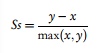 (4)
where x denotes the mean distance between a specific data point and other points in its cluster, and y indicates the mean distance from that same point to the nearest points in the adjacent cluster. The resulting anomalous points identified using optimized DBSCAN parameters are illustrated in Figure 8 for the four datasets.
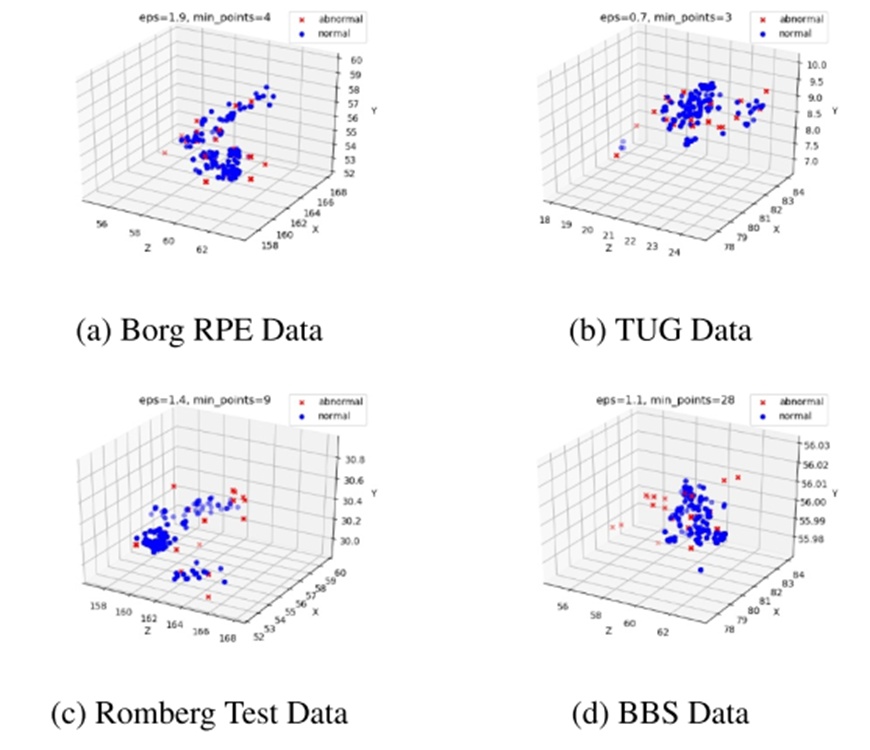
Figure 8. Visualisation of abnormal detection with optimised density-based spatial clustering of applications with noise parameters.
In addition to optimizing DBSCAN parameters, we introduce a hybrid approach that incorporates the IQR for further anomaly detection. After clustering data points using the optimized DBSCAN, we identify outliers by locating points residing outside the IQR thresholds. The IQR is computed using Eq. 5:
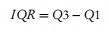 (5)
In this context, Q_1 represents the first quartile (lower), and Q_3 represents the third quartile (upper). Outliers are defined as data points falling outside the range [Q1 - k ∗ IQR, Q3 + k ∗ IQR], where k is a user-defined constant.
The hybrid anomaly detection method integrates the optimized DBSCAN clustering with the IQR-based outlier identification. The hybrid abnormality score H is computed by combining the silhouette score S (from DBSCAN) and the outlier score from the IQR, adjusted by a weight W.
The final equation for the hybrid abnormality detection is given in Eq. 6:
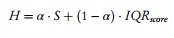 (6)
In this formula, S is the silhouette score derived from the optimized DBSCAN algorithm, and IQRscore is the outlier score obtained from the IQR method. The parameter α [0, 1] is a user-defined weight that regulates the relative importance of the DBSCAN clustering (S) and the IQR-based detection (IQRscore). A higher \alpha prioritizes the DBSCAN results, while a lower \alpha assigns greater significance to the IQR-based identification. A visual representation of anomaly detection for all four datasets using the Hybrid Abnormal Detection with Optimized DBSCAN and IQR is provided in Figure 9.
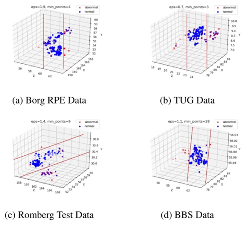
Figure 9. Visualisation of hybrid abnormal detection with optimised density-based spatial clustering of applications with noise and interquartile range.
The primary objective of this chapter is to quantify the proficiency of the regression frameworks in projecting the study's target variable. We determine algorithmic exactness by contrasting the generated forecasts directly against empirical, real-world data. To appropriately measure the success of each trial, we apply standard evaluation parameters—chiefly the R2 coefficient alongside diverse error-based statistics—to characterize the operational quality of the models.
Machine learning relies on regression techniques to map the correlations distinguishing independent inputs from a dependent output. At its core, this statistical approach is designed to project continuous, distinct quantitative measures, encompassing domains like market pricing, energy expenditure, or user scoring.
Within healthcare environments, clinical specialists utilize a spectrum of performance criteria to confirm the exactness and dependability of predictive systems. Statistical yardsticks—specifically MAE, MSE, RMSE, R2, RMSLE, and MAPE—deliver critical perspective on the algorithm's forecasting power. To illustrate, absolute and squared metrics (MAE, MSE, RMSE) define the absolute magnitude of predictive deviation, whereas the R2 value expresses the fraction of variance successfully accounted for by the mathematical model. Furthermore, RMSLE is exceptionally suited for wide-ranging numerical distributions, and MAPE calculates predictive precision proportionally to the true baseline values. By thoroughly decoding these diagnostic metrics, medical practitioners can formulate sound conclusions regarding algorithmic validity, ensuring these tools are appropriately integrated into patient care protocols and clinical decision-support platforms.
R2 Score: A standard benchmark for determining the success of machine learning regression is the R2 score, which acts as a primary barometer for algorithmic goodness-of-fit. Formally termed the coefficient of determination, this metric elucidates the proportion of data variability captured by the system's forecasts. The mathematical derivation for the R2 score is outlined in Eq. 7:
 (7)
In this formulation, SSR symbolizes the sum of squared discrepancies separating forecasted and actual values, while SSt represents the overall squared variance of all data points relative to the sample mean. The R2 coefficient spans a scale from 0 to 1 and is frequently expressed in percentage form.
MAE: Mean Absolute Error operates as an evaluation tool that computes the mean of the absolute discrepancies separating empirical observations from algorithmic forecasts. It delivers a highly intuitive gauge of predictive proximity to actual dataset values. To conceptualize this, consider a model supplied with paired input-output features where linear regression calculates the optimal trajectory. Determining the MAE requires identifying instances of predictive divergence, recognized mathematically as errors. Once the gap separating true and forecasted outcomes is established, the absolute discrepancies are aggregated across the entire dataset and divided by the total instance count. This final calculation represents the overarching loss value, which developers continuously strive to minimize. The mathematical computation for MAE is detailed below in Eq. 8:
 (8)
Within this expression, yi stands for the empirical ground truth data, defines the algorithm's projection, and x indicates the aggregate count of data samples. Driving down the MAE remains a fundamental objective throughout a vast array of predictive and regression-based applications.
MSE: Mean Squared Error serves as another prevalent evaluation tool, offering a nuanced alternative to MAE. The fundamental distinction centers on its mathematical execution: MSE squares the deviation separating actual and forecasted outcomes, intentionally magnifying the penalty for larger discrepancies. Consequently, while MAE captures pure absolute variance, MSE calculates the average of these squared deviations. A key mathematical benefit of squaring these terms is the elimination of negative values, preventing opposing errors from neutralizing one another. The formalized calculation for MSE is provided in Eq. 9:
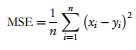 (9)
According to Eq. 9, yi reflects the projections outputted by the trained architecture, xi stands for the true target variables within the corpus, and n corresponds to the total instances processed.
RMSE: Root Mean Squared Error offers particular utility when analyzing how forecasting errors are distributed relative to the empirical baseline. A minimized RMSE confirms that the algorithmic outputs tightly cluster around the true observational coordinates. In contrast, an inflated RMSE implies a substantially larger average deviation. The systematic methodology for deriving the RMSE is outlined in Eq. 10.
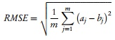 (10)
In Eq. 10, bj corresponds to the algorithmic prediction, aj represents the empirical target present in the dataset, and m signifies the comprehensive total of dataset records.
MAPE: Mean Absolute Percentage Error acts as a specialized instrument for determining the reliability of forecasting algorithms. It measures the mean proportional divergence separating the projected outcomes from the empirical reality. Because it is formulated as a percentage, MAPE is inherently intuitive to read and analyze. The mathematical representation for MAPE is detailed in Eq. 11.
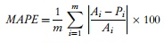 (11)
where m denotes the total pool of data entries. The variable Ai signifies the true baseline figure for a specific data point i, whereas Pi represents the corresponding forecasted value for that same point i.
This segment is dedicated to visualizing the juxtaposition of real versus forecasted values across four distinct pathology datasets. Furthermore, we evaluate the comparative impact of anomaly elimination using three distinct techniques: the standard DBSCAN algorithm configured with parameters derived from the reference literature [61], a fine-tuned version of DBSCAN, and ultimately, an optimized DBSCAN paired with the Interquartile Range (IQR)—which constitutes the novel abnormal detection framework introduced in this research.
In this initial scenario, we map the baseline results derived from the raw data to observe intrinsic patterns prior to the extraction of any irregular anomalies. Under these conditions, the four target datasets—Borg RPE, TUG, Romgberg test, and BBS—are processed through LGB, XGB, RF, and AutoML forecasting models. Figure 10 is divided into four distinct panels, designated Figure 10a–d. Specifically, Figure 10a portrays the empirical versus forecasted trajectories for the Borg RPE dataset applying all four frameworks. The actual baseline coordinates are plotted using a solid blue line; the LGB projections are marked by a dash-dotted orange trace; the XGB outputs by a dotted green path; the RF estimates by a dash-dotted red line; and the AutoML forecasts are represented by a dotted purple trace. Observing the Borg RPE outcomes in Figure 10a, the predictive fidelity of all algorithms is robust, although the underlying solid blue trace remains exposed at certain peak instances. In contrast, Figure 10b reveals that the TUG disease forecasts yield only moderate accuracy, as a substantial number of projections deviate noticeably beyond the reference line. Regarding the Romgberg test dataset evaluated in Figure 10c, the algorithms demonstrate high accuracy across intermediate ranges but exhibit clear shortcomings when modeling peak values, leaving the solid empirical baseline visible. Finally, examining the BBS disease data in Figure 10d, the forecasting architectures frequently fail to track the blue trajectory, generating predictions that overshoot the true baseline.
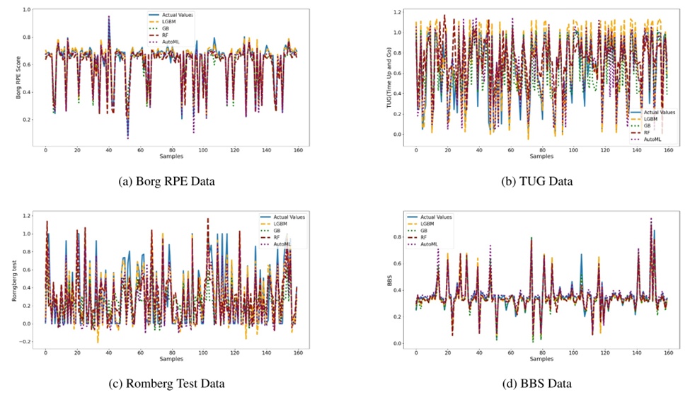
Figure 10. Actual and predicted data visualisation before abnormal detection. AutoML, automated machine learning; BBS, Berg Balance Scale; RF, random forest.
Here, we analyze the ramifications of executing the DBSCAN framework utilizing the specific configurations defined in the reference literature [61] to detect and filter out anomalous records. The primary goal is to evaluate how this specific data-preprocessing mechanism alters the forecasting efficacy of the four machine learning architectures across the Borg RPE, TUG, Romberg Test, and BBS datasets. Figure 11 illustrates the true versus projected trajectories for all four conditions following the implementation of DBSCAN governed by the parameters sourced from study [61].
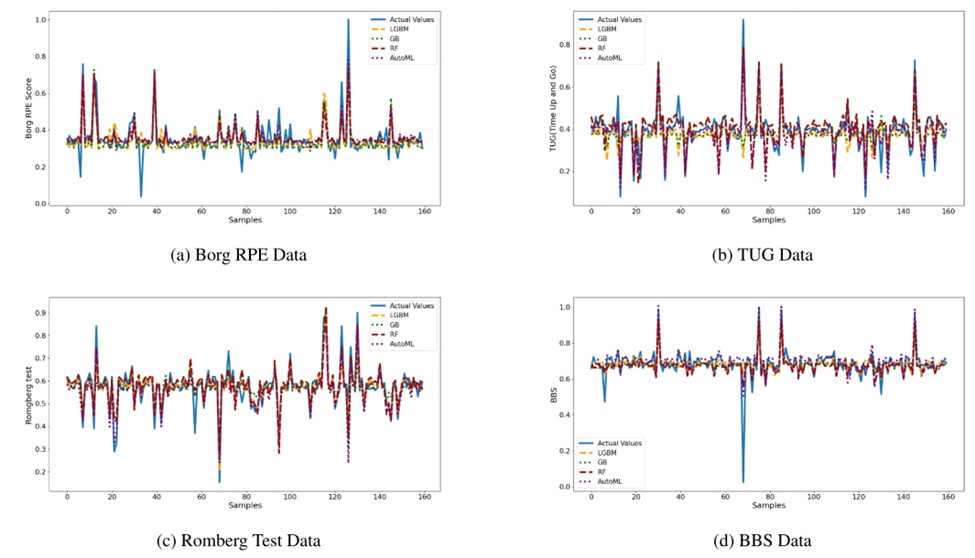
Figure 11. Actual and predicted data visualisation after AD with density-based spatial clustering of applications with noise using referenced paper parameters [61]. AutoML, automated machine learning; BBS, Berg Balance Scale; RF, random forest.
It is critical to emphasize that, as the analysis indicates, the empirical findings fail to match the promise of the earlier trials. Applying the DBSCAN technique with these specific constraints inadvertently eliminated a massive proportion of legitimate, non-abnormal records, causing a corresponding deterioration in algorithmic forecasting power. This degradation is vividly apparent when examining the visual plots provided in Figures 11a–11d. Ultimately, this section underscores the profound influence of the DBSCAN preprocessing phase, drawing attention to the delicate trade-off between aggressively filtering outliers and potentially sacrificing overall predictive reliability.
This final segment probes the consequences of applying a refined set of DBSCAN parameters—isolated via grid search optimization—to actively identify and discard dataset anomalies. The core objective is to gauge how this upgraded preprocessing methodology augments the predictive capability of the four ML models across the Borg RPE, TUG, Romberg Test, and BBS data cohorts. Figures 12a–12d chart the empirical versus projected outcomes for all four target variables subsequent to the application of the fine-tuned DBSCAN protocol. This upgraded data-cleaning workflow demonstrably elevates forecasting accuracy when benchmarked against prior experiments. Despite this improvement, it is important to acknowledge that the predictive models occasionally fall short of perfectly mirroring the empirical data trace (the blue line).
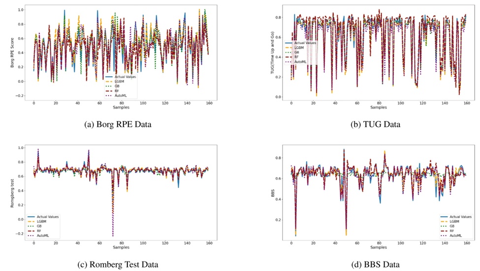
Figure 12. Actual and predicted data visualisation after AD with optimised density-based spatial clustering of applications with noise. AutoML, automated machine learning; BBS, Berg Balance Scale; RF, random forest.
This portion of the analysis clearly demonstrates the tangible benefits of calibrating DBSCAN configurations to elevate the data-preprocessing workflow. Even with these enhancements, the algorithms continue to encounter localized challenges in reproducing highly specific nuances embedded within the feature space, an issue prominently visible when inspecting the comparative visual graphs, most notably in Figure 12a.
The forecasted versus empirical outcomes across the four distinct disease categories, subsequent to implementing the newly introduced hybrid anomaly detection framework, are depicted in Figure 13.
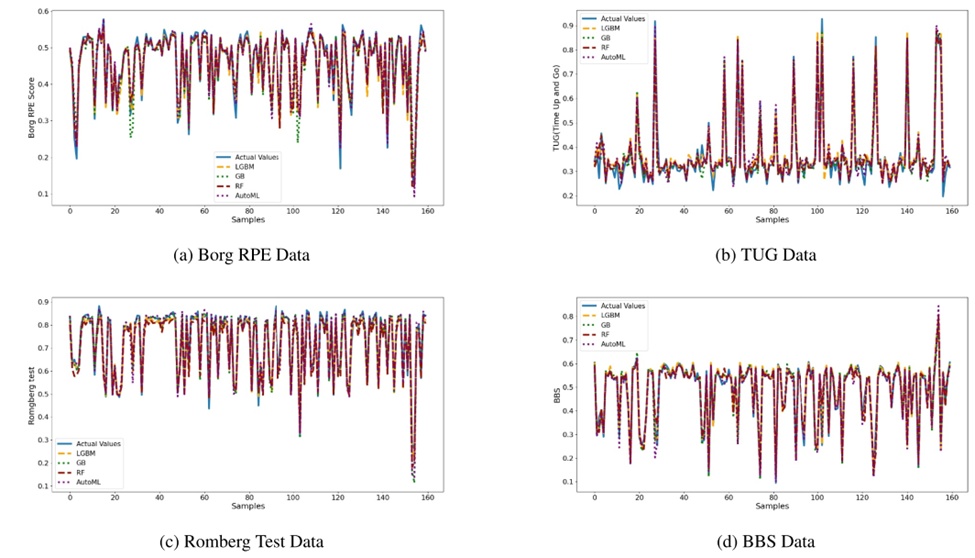
Figure 13. Actual and predicted data visualisation after AD with proposed Hybrid AD model. AutoML, automated machine learning; BBS, Berg Balance Scale; RF, random forest.
These graphical plots clearly demonstrate the effectiveness of the introduced hybrid strategy for isolating anomalies. A strong convergence between the forecasted coordinates and the true observations highlights the advanced capability of this detection framework. Such tight alignment confirms that the hybrid architecture successfully elevates overall dataset integrity by accurately isolating and discarding irregular instances.
Additionally, the findings indicate that the secondary framework introduced in this study, AutoML, yields superior forecasting power when benchmarked against prominent algorithms like LGB, XGB, and RF. The exceptional tracking of the empirical baseline by the generated projections visually confirms AutoML's proficiency in modeling complex internal data relationships.
Ultimately, deploying the hybrid anomaly filtration mechanism—merging the Interquartile Range (IQR) with optimally tuned DBSCAN configurations—yields a massive gain in forecasting precision. Moreover, utilizing AutoML as a core predictive engine highlights its immense utility for robust model selection and hyperparameter optimization (HPO).
During the rigorous evaluation of the VP0004 Borg RPE dataset, multiple machine learning architectures underwent performance testing across diverse anomaly filtering configurations, with the outcomes detailed in Table 2.
Evaluating the baseline VP0004 data, AutoML continually emerged as the dominant algorithm, achieving the maximum R2 score (0.9713) while securing the minimum RMSE, MSE, and MAE metrics. The LGB architecture also produced strong outcomes, notably registering an R2 of 0.9599 and an RMSE of 0.0474. Implementing the DBSCAN protocol governed by the reference literature parameters did not disrupt this hierarchy; AutoML attained an R2 of 0.858, an RMSE of 0.051, and an MAE of 0.031, whereas both XGB and LGB continued to show robust viability.
When applying fine-tuned DBSCAN configurations to the VP0004 cohort, AutoML again surpassed alternative models, logging a strong R2 of 0.974 alongside an RMSE of 0.033 and an MAE of 0.015. This dominance was equally evident when evaluating the dataset processed via the hybrid framework (optimized DBSCAN merged with IQR), where AutoML recorded a stellar R2 of 0.998, an RMSE of 0.030, and the lowest overall MAE (0.013). Throughout these successive trials, the XGB and LGB frameworks consistently retained competitive efficacy.
Table 2. Performance comparison of ML models in abnormal detection for VP0004 Borg RPE dataset.
AD techniques | MAPE | RMSLE | R2 | RMSE | MSE | MAE | Models |
VP0004 | 0.0778 | 0.0306 | 0.9599 | 0.0474 | 0.0026 | 0.0222 | LGB |
0.0742 | 0.0273 | 0.9696 | 0.0422 | 0.0019 | 0.0234 | XGB | |
0.0759 | 0.0306 | 0.9633 | 0.0469 | 0.0024 | 0.0257 | RF | |
0.0657 | 0.0267 | 0.9713 | 0.0415 | 0.0019 | 0.0216 | AutoML | |
VP0004 (DBSCAN paper parameters) | 0.10 | 0.045 | 0.805 | 0.071 | 0.005 | 0.035 | LGB |
0.093 | 0.040 | 0.820 | 0.058 | 0.004 | 0.034 | XGB | |
0.105 | 0.046 | 0.798 | 0.071 | 0.005 | 0.037 | RF | |
0.085 | 0.038 | 0.858 | 0.051 | 0.003 | 0.031 | AutoML | |
VP0004 (DBSCAN optimise parameters) | 0.070 | 0.023 | 0.965 | 0.040 | 0.0012 | 0.018 | LGB |
0.067 | 0.021 | 0.970 | 0.035 | 0.0011 | 0.017 | XGB | |
0.072 | 0.024 | 0.963 | 0.041 | 0.0013 | 0.019 | RF | |
0.065 | 0.020 | 0.974 | 0.033 | 0.001 | 0.015 | AutoML | |
VP0004 hybrid (optimal DBSCAN + IQR) | 0.057 | 0.018 | 0.976 | 0.035 | 0.0012 | 0.015 | LGB |
0.055 | 0.016 | 0.982 | 0.032 | 0.0010 | 0.014 | XGB | |
0.060 | 0.018 | 0.975 | 0.036 | 0.0013 | 0.016 | RF | |
0.052 | 0.015 | 0.998 | 0.030 | 0.0009 | 0.013 | AutoML |
Note: Bold values in the results Tables showing the Proposed model highest results.
Abbreviations: AutoML, automated machine learning; BBS, Berg Balance Scale; DBSCAN, density-based spatial clustering of applications with noise; IQR, interquartile range; LGB, light GB; MAE, mean absolute error; MAPE, mean absolute percentage error; MSE, mean squared error; RF, random forest; RMSE, root mean squared error; RMSLE, root mean squared logarithmic error; RPE, rating of perceived exertion; XGB, XGBoost.
To synthesize, although the diverse machine learning algorithms crucially verified the anomaly filtration techniques, the central objective is the appraisal of the detection methodologies themselves. The ideal framework will ultimately depend upon unique project demands and inherent data traits. Nevertheless, the combined strategy of IQR and calibrated DBSCAN undeniably stands out as the superior anomaly isolation tool for the VP0004 dataset.
Table 3 outlines the comprehensive assessment of multiple machine learning algorithms applied to the VP0005 TUG dataset, aiming to benchmark their capabilities under various anomaly elimination protocols.
When processing the raw VP0005 dataset, AutoML definitively outperformed the group by securing the peak R2 parameter (0.948) alongside the lowest RMSE, MSE, and MAE scores. Concurrently, the LGB algorithm demonstrated solid capability, highlighted by an R2 of 0.950 and an RMSE of 0.052. This hierarchy held steady following the application of DBSCAN configured with parameters from the cited literature. In this condition, AutoML registered an R2 of 0.948, an RMSE of 0.0598, and an MAE of 0.0598, with the XGB and LGB frameworks closely trailing.
Table 3. Performance comparison of ML models in abnormal detection for VP0005 TUG dataset.
Data | Models | MAPE | RMSLE | R2 | RMSE | MSE | MAE |
VP0005 | LGB | 0.0521 | 0.045 | 0.950 | 0.052 | 0.003 | 0.026 |
XGB | 0.068 | 0.044 | 0.952 | 0.051 | 0.003 | 0.027 | |
RF | 0.0598 | 0.048 | 0.948 | 0.054 | 0.003 | 0.028 | |
AutoML | 0.0519 | 0.044 | 0.948 | 0.0598 | 0.0598 | 0.0598 | |
VP0005 (DBSCAN paper parameters) | LGB | 0.090 | 0.036 | 0.925 | 0.065 | 0.004 | 0.028 |
XGB | 0.085 | 0.033 | 0.936 | 0.052 | 0.003 | 0.027 | |
RF | 0.095 | 0.038 | 0.920 | 0.068 | 0.004 | 0.030 | |
AutoML | 0.075 | 0.030 | 0.954 | 0.046 | 0.023 | 0.023 | |
VP0005 (DBSCAN optimise parameters) | LGB | 0.075 | 0.030 | 0.941 | 0.047 | 0.0022 | 0.022 |
XGB | 0.070 | 0.028 | 0.951 | 0.044 | 0.0019 | 0.021 | |
RF | 0.080 | 0.032 | 0.936 | 0.049 | 0.0024 | 0.024 | |
AutoML | 0.065 | 0.026 | 0.958 | 0.040 | 0.0016 | 0.019 | |
VP0005 hybrid (optimal DBSCAN + IQR) | LGB | 0.055 | 0.017 | 0.963 | 0.040 | 0.0016 | 0.021 |
XGB | 0.052 | 0.016 | 0.975 | 0.036 | 0.0013 | 0.020 | |
RF | 0.057 | 0.018 | 0.961 | 0.042 | 0.0018 | 0.022 | |
AutoML | 0.050 | 0.015 | 0.993 | 0.034 | 0.0012 | 0.019 |
Note: Bold values in the results Tables showing the Proposed model highest results.
Abbreviations: AutoML, automated machine learning; BBS, Berg Balance Scale; DBSCAN, density-based spatial clustering of applications with noise; IQR, interquartile range; LGB, light GB; MAE, mean absolute error; MAPE, mean absolute percentage error; MSE, mean squared error; RF, random forest; RMSE, root mean squared error; RMSLE, root mean squared logarithmic error; XGB, XGBoost.
Examining the VP0005 data cleaned via fine-tuned DBSCAN constraints, AutoML again exceeded alternative architectures, obtaining an R2 of 0.958, an RMSE of 0.040, and an MAE of 0.019. The LGB algorithm provided comparable reliability, achieving an R2 of 0.941 and an RMSE of 0.047. Merging the IQR technique with the calibrated DBSCAN framework proved highly beneficial for AutoML, securing its rank as the premier model by recording the minimum RMSE (0.034), the lowest MAE (0.019), and a remarkable R2 (0.993). Throughout these trials, the LGB algorithm consistently proved to be a formidable contender.
The overarching goal of this investigation is identifying the optimal outlier filtration strategy tailored to the VP0005 TUG records, heavily weighing systemic demands and statistical features. Although the predictive algorithms were instrumental in testing these paradigms, assessing the detection strategies takes precedence. Optimal selections invariably depend on the specific cohort in question; however, the data confirms that integrating IQR with a calibrated DBSCAN architecture provides the most robust anomaly identification for the VP0005 corpus.
A thorough appraisal of anomaly identification on the VP0006 Romberg Test data is outlined in Table 4. The predictive frameworks display fluctuating performance levels across distinct experimental conditions, encompassing both IQR integration and modified DBSCAN constraints. Throughout these iterations, AutoML reliably secures the peak R2 measurements and the lowest RMSE statistics, underscoring its profound ability to model the VP0006 feature space. Additionally, these findings highlight the critical nature of parameter tuning, given that all algorithms demonstrate enhanced accuracy when driven by optimized DBSCAN thresholds.
Table 4. Performance comparison of ML models in abnormal detection for Romgberg Test: VP0006 dataset.
Data | Models | MAPE | RMSLE | R2 | RMSE | MSE | MAE |
VP0006 | LGB | 0.0763 | 0.0313 | 0.961 | 0.055 | 0.003 | 0.044 |
XGB | 0.0758 | 0.0317 | 0.96 | 0.056 | 0.0032 | 0.046 | |
RF | 0.0747 | 0.032 | 0.959 | 0.058 | 0.0034 | 0.048 | |
AutoML | 0.0772 | 0.0315 | 0.962 | 0.054 | 0.0031 | 0.042 | |
VP0006 (DBSCAN paper parameters) | LGB | 0.085 | 0.036 | 0.931 | 0.067 | 0.0046 | 0.056 |
XGB | 0.087 | 0.0365 | 0.928 | 0.070 | 0.0049 | 0.058 | |
RF | 0.089 | 0.037 | 0.925 | 0.071 | 0.0051 | 0.060 | |
AutoML | 0.084 | 0.035 | 0.933 | 0.065 | 0.0043 | 0.054 | |
VP0006 (DBSCAN optimise parameters) | LGB | 0.065 | 0.020 | 0.962 | 0.034 | 0.0012 | 0.018 |
XGB | 0.062 | 0.019 | 0.970 | 0.031 | 0.0010 | 0.017 | |
RF | 0.068 | 0.021 | 0.961 | 0.036 | 0.0013 | 0.019 | |
AutoML | 0.060 | 0.018 | 0.974 | 0.032 | 0.0010 | 0.016 | |
VP0006 hybrid (optimal DBSCAN + IQR) | LGB | 0.055 | 0.016 | 0.971 | 0.036 | 0.0013 | 0.019 |
XGB | 0.053 | 0.015 | 0.987 | 0.034 | 0.0012 | 0.018 | |
RF | 0.052 | 0.014 | 0.985 | 0.033 | 0.0011 | 0.018 | |
AutoML | 0.050 | 0.014 | 0.999 | 0.032 | 0.0010 | 0.016 |
Note: Bold values in the results Tables showing the Proposed model highest results.
Abbreviations: AutoML, automated machine learning; BBS, Berg Balance Scale; DBSCAN, density-based spatial clustering of applications with noise; IQR, interquartile range; LGB, light GB; MAE, mean absolute error; MAPE, mean absolute percentage error; MSE, mean squared error; RF, random forest; RMSE, root mean squared error; RMSLE, root mean squared logarithmic error; XGB, XGBoost.
Substantial boosts in predictive capacity are noted universally across all algorithms when subjected to the calibrated DBSCAN workflow. To illustrate, AutoML secures a striking R2 of 0.974 and an RMSE of 0.032, surpassing the LGB model, which registers an R2 of 0.962 and an RMSE of 0.034. Fusing the IQR methodology with the fine-tuned DBSCAN setup amplifies detection precision even further. Under this hybrid protocol, AutoML dominates by achieving an unparalleled R2 of 0.999 alongside an RMSE of 0.032, reflecting a nearly flawless predictive alignment. Ultimately, these outcomes emphasize how algorithm calibration and sophisticated hybrid models drastically augment anomaly filtration within the VP0006 dataset.
When applying varied DBSCAN iterations and IQR techniques to isolate outliers in the VP0007 BBS dataset, the forecasting algorithms display unique behavioral traits. Optimizing the DBSCAN configuration universally translates into marked improvements in algorithmic accuracy. Specifically, AutoML commands an outstanding R2 of 0.968 and an RMSE of 0.037, eclipsing the LGB framework's strong RMSE of 0.043 and R2 of 0.952. Unifying the IQR protocol with the calibrated DBSCAN architecture triggers even greater leaps in filtration accuracy. Employing this hybrid setup, AutoML achieves a phenomenal R2 of 0.997 and an RMSE of 0.030, denoting an essentially absolute correlation with the target variables. These metrics validate the power of rigorous parameter tuning and complex methodologies to heavily upgrade outlier identification for the VP0007 cohort. Table 5 provides the exhaustive metrics for the VP0007 BBS trial.
Table 5. Performance comparison of ML models in abnormal detection for BBS: VP0007 dataset.
Data | Models | MAPE | RMSLE | R2 | RMSE | MSE | MAE |
VP0007 | LGB | 0.085 | 0.040 | 0.935 | 0.0671 | 0.0045 | 0.061 |
XGB | 0.082 | 0.038 | 0.915 | 0.0632 | 0.004 | 0.055 | |
RF | 0.079 | 0.036 | 0.925 | 0.0608 | 0.0037 | 0.049 | |
AutoML | 0.076 | 0.034 | 0.942 | 0.0575 | 0.0033 | 0.043 | |
VP0007 (DBSCAN paper parameters) | LGB | 0.072 | 0.026 | 0.931 | 0.047 | 0.0022 | 0.028 |
XGB | 0.071 | 0.025 | 0.936 | 0.046 | 0.0021 | 0.027 | |
RF | 0.074 | 0.027 | 0.932 | 0.048 | 0.0023 | 0.029 | |
AutoML | 0.068 | 0.023 | 0.954 | 0.042 | 0.0018 | 0.025 | |
VP0007 (DBSCAN optimise parameters) | LGB | 0.065 | 0.021 | 0.952 | 0.043 | 0.0018 | 0.022 |
XGB | 0.062 | 0.020 | 0.959 | 0.040 | 0.0016 | 0.021 | |
RF | 0.068 | 0.022 | 0.950 | 0.045 | 0.0020 | 0.024 | |
AutoML | 0.059 | 0.019 | 0.968 | 0.037 | 0.0014 | 0.019 | |
VP0007 hybrid (optimal DBSCAN + IQR) | LGB | 0.052 | 0.015 | 0.970 | 0.033 | 0.0011 | 0.017 |
XGB | 0.050 | 0.014 | 0.985 | 0.032 | 0.0010 | 0.017 | |
RF | 0.053 | 0.016 | 0.975 | 0.034 | 0.0012 | 0.018 | |
AutoML | 0.048 | 0.013 | 0.997 | 0.030 | 0.0009 | 0.015 |
Note: Bold values in the results Tables showing the Proposed model highest results.
Abbreviations: AutoML, automated machine learning; BBS, Berg Balance Scale; DBSCAN, density-based spatial clustering of applications with noise; IQR, interquartile range; LGB, light GB; MAE, mean absolute error; MAPE, mean absolute percentage error; MSE, mean squared error; RF, random forest; RMSE, root mean squared error; RMSLE, root mean squared logarithmic error; XGB, XGBoost.
This chapter critically unpacks the broader consequences and effectiveness of the study, underscoring its academic value and core contributions. By benchmarking our results against established literature on anomaly identification, we emphasize the detrimental toll that irregular observations exact on algorithmic precision. Eliminating these anomalous records structurally fortifies the model, minimizing bias and statistical noise to yield superior forecasting and generalization capabilities. The empirical data strongly corroborates these efficiency gains, spotlighting the undeniable necessity of rigorous data cleaning mechanisms, notably outlier filtration. To comprehensively measure algorithmic success, critical statistical tools such as MAPE and the R2 coefficient are rigorously analyzed.
The preliminary phase of this discussion concentrates on tracking empirical gains specifically measured via the R2 metric. Figure 14 is presented as a graphical reference mapping the upward progression of forecasting precision, thereby delivering a holistic perspective on the improvements driven by the introduced pipeline.
Panel 14a graphically compares the outcomes for the Borg RPE cohort. The preliminary testing on the unaltered data provided baseline R2 benchmarks for AutoML (0.971), XGB (0.969), RF (0.963), and LGB (0.959). When filtering anomalies using DBSCAN configurations sourced from Study [2], the frameworks experienced an overt shift in forecasting capability. Specifically, AutoML suffered a prominent 0.113 drop, retreating from 0.971 down to 0.858. Corresponding performance declines manifested across the RF (0.165), LGB (0.154), and XGB (0.151) architectures. This phenomenon highlights that while the cleaning mechanism aggressively filtered data, it triggered an unavoidable contraction in baseline R2 values.
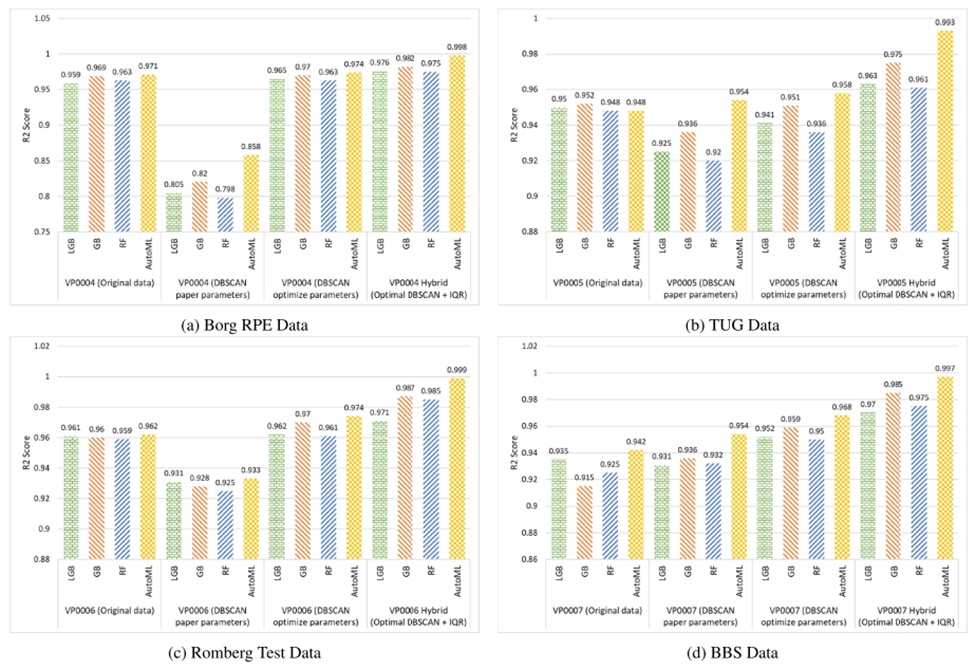
Figure 14. Four clinical data Rscore analyses in different abnormal detection scenarios. AutoML, automated machine learning; BBS, Berg Balance Scale; DBSCAN, density-based spatial clustering of applications with noise; IQR, interquartile range; RF, random forest.
Progressing further, fine-tuning the DBSCAN threshold parameters stimulated renewed predictive gains. AutoML successfully rebounded, eclipsing its raw data baseline by 0.003 to attain an R2 of 0.974. In parallel, the RF, LGB, and XGB models recorded marginal uplifts of 0.012, 0.006, and 0.001, respectively, denoting subtle enhancements beyond the uncleaned dataset. The critical breakthrough arrived upon deploying the hybrid mechanism, merging IQR with the calibrated DBSCAN. Under this setup, AutoML surged to a formidable R2 of 0.998, marking a massive 0.027 escalation above the baseline. The remaining algorithms—LGB (0.017), XGB (0.013), and RF (0.012)—similarly recorded marked leaps, powerfully demonstrating the synergistic benefits of the composite filtration framework over the raw dataset.
Summing up the absolute gains separating the baseline Borg RPE records from the novel hybrid framework, AutoML achieved a net R2 increase of 0.027. Concurrently, the LGB, XGB, and RF models accrued total advancements of 0.017, 0.013, and 0.012, respectively. These statistics validate the overarching methodology's success in fortifying algorithm stability and projection accuracy, successfully navigating the initial R2 penalties encountered during the early stages of data sanitization.
Shifting to the TUG dataset illustrated in Figure 14b, preliminary trials generated baseline R2 coefficients for the XGB (0.952), LGB (0.950), AutoML (0.948), and RF (0.948) architectures. Filtering the cohort using DBSCAN constraints sourced from external literature instigated pronounced shifts. Demonstrating high tolerance to outlier extraction, AutoML actually improved its R2 metric by 0.006 over the raw baseline. Conversely, the RF (0.026), LGB (0.025), and XGB (0.024) algorithms all suffered R2 degradations, underscoring the inherent compromise between rigorous data purging and the retention of baseline forecasting power for these specific models.
Calibrating the DBSCAN parameters prompted fragmented improvements. AutoML recorded a notable R2 surge of 0.010 above the uncleaned baseline, settling at 0.958. Conversely, the RF, LGB, and XGB algorithms still recorded deficits of 0.012, 0.009, and 0.001 compared to the original data. These contrasting trajectories emphasize the complex ramifications data scrubbing imposes on distinct predictive algorithms. A dramatic turning point occurred upon executing the integrated IQR and calibrated DBSCAN protocol. Under this hybrid configuration, AutoML skyrocketed to an R2 of 0.993, representing a remarkable 0.045 gain over the baseline data. The XGB (0.023), LGB (0.013), and RF (0.013) architectures likewise secured positive net growth.
Tallying the total performance delta between the unprocessed TUG corpus and the final hybrid architecture reveals a cumulative 0.045 R2 enhancement for AutoML. Simultaneously, the XGB, LGB, and RF frameworks locked in total net improvements of 0.023, 0.013, and 0.013, respectively. Ultimately, these findings heavily reinforce the value of the composite methodology in elevating algorithmic durability for the TUG dataset, efficiently mitigating the initial metric penalties tied to aggressive anomaly extraction.
The results presented in Figure 14c highlight the substantial gains in predictive capability achieved by applying the novel anomaly detection strategy to the Romberg test dataset. In their baseline state, the LGB, XGB, RF, and AutoML architectures yielded R2 metrics of 0.961, 0.96, 0.959, and 0.962, respectively. The deployment of DBSCAN configured with parameters from Ref. [61] caused a severe degradation in forecasting power. Conversely, modifying the DBSCAN configuration via parameter optimization generated a distinct improvement. In particular, the R2 values experienced slight upward shifts of 0.001 for LGB, 0.01 for XGB, 0.002 for RF, and 0.012 for AutoML relative to the uncleaned baseline. This confirms the value and exactness of targeted anomaly extraction for boosting algorithm precision. Progressing further, the optimized DBSCAN protocol was combined with IQR to sanitize the Romberg test records. The ensuing outcomes were highly impressive, most notably for AutoML, which secured a massive 0.037 R2 gain over the raw data to achieve a remarkable 0.999. Similarly, the alternative algorithms experienced notable forecasting improvements under this integrated anomaly filtration methodology, confirming its exceptional capacity to fortify predictive stability for Romberg test data.
Figure 14d visualizes how the anomaly isolation protocol influences forecasting models operating on the BBS dataset. Baseline R2 coefficients for the LGB, XGB, RF, and AutoML frameworks registered at 0.935, 0.915, 0.925, and 0.942, respectively. Executing DBSCAN governed by literature-sourced parameters generated complex fluctuations: LGB dropped marginally to 0.931 (−0.004), while XGB climbed to 0.936 (+0.021), RF increased to 0.932 (+0.007), and AutoML surged to 0.954 (+0.012). These variations emphasize the complex consequences of DBSCAN-based data sanitization. Calibrating the DBSCAN configuration universally elevated performance. LGB grew to 0.952 (+0.017), XGB reached 0.959 (+0.044), RF advanced to 0.95 (+0.025), and AutoML expanded to 0.968 (+0.026), proving that parameter tuning successfully bolsters forecasting exactness. Merging this optimized DBSCAN structure with the IQR technique triggered even greater gains. LGB hit 0.97 (+0.035), XGB peaked at 0.985 (+0.07), RF advanced to 0.975 (+0.05), and AutoML dominated at 0.997 (+0.055). Measuring the net progression from the uncleaned BBS records to the final composite framework, AutoML recorded an exceptional aggregate growth of 0.055, while the LGB, XGB, and RF architectures accumulated total enhancements of 0.035, 0.07, and 0.05, respectively. Such outcomes powerfully validate the anomaly extraction protocol's capacity to amplify algorithmic durability for the BBS cohort, carefully navigating the initial metric compromises inherent to data purging.
Transitioning our analytical focus to the MAPE, we conduct an extensive evaluation of algorithmic stability beyond the confines of the R2 metric. This deeper probe yields valuable context regarding the operational success of the anomaly filtration strategy across heterogeneous clinical cohorts. The comparative visualizations detailed in Figure 15 highlight how this methodology influences the MAPE, elucidating the study's broader consequences for elevating both forecasting precision and overall system dependability.
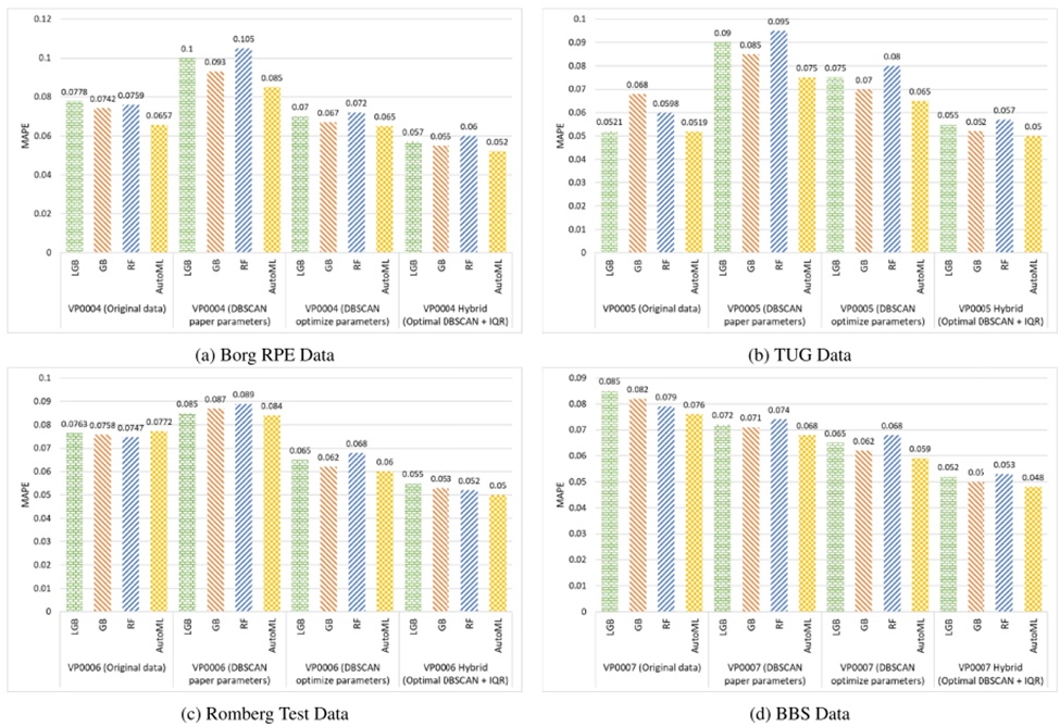
Figure 15. Analysing mean absolute percentage error errors in clinical data prediction in different abnormal detection mechanisms. AutoML, automated machine learning; BBS, Berg Balance Scale; DBSCAN, density-based spatial clustering of applications with noise; IQR, interquartile range; RF, random forest.
Panel 15a illustrates the baseline MAPE statistics for the raw Borg RPE dataset, where the LGB, XGB, RF, and AutoML frameworks registered at 0.0778, 0.0742, 0.0759, and 0.0657, respectively. The deployment of DBSCAN utilizing literature-derived configurations to isolate anomalies triggered a marked escalation in predictive divergence universally: LGB surged to 0.1 (+0.022), XGB climbed to 0.093 (+0.018), RF spiked to 0.105 (+0.029), and AutoML advanced to 0.085 (+0.019). Following this, calibrating the DBSCAN parameters prompted uniform reductions in the MAPE relative to the raw baseline: LGB fell to 0.07 (−0.007), XGB contracted to 0.067 (−0.007), RF dropped to 0.072 (−0.004), and AutoML shrank to 0.065 (−0.001). Unifying this calibrated DBSCAN model with the IQR methodology generated even more dramatic error minimization: LGB plunged to 0.057 (−0.021), XGB shrank to 0.055 (−0.019), RF lowered to 0.06 (−0.016), and AutoML plummeted to 0.052 (−0.014). These metrics definitively confirm the continuous gains in predictive exactness and loss mitigation facilitated by the anomaly filtration protocol on the Borg RPE records.
Evaluating the TUG dataset as depicted in Figure 15b, the analysis initiates by reviewing the uncleaned MAPE baseline metrics for the LGB, XGB, RF, and AutoML forecasting tools, which recorded at 0.0521, 0.068, 0.0598, and 0.0519, respectively. These preliminary figures function as the reference point for evaluating downstream anomaly filtration methods. Executing DBSCAN with literature-based constraints to purge irregularities caused conspicuous fluctuations in predictive loss. LGB suffered a severe escalation, hitting a MAPE of 0.09 (+0.0379), while the XGB, RF, and AutoML architectures similarly ballooned to 0.085 (+0.017), 0.095 (+0.0352), and 0.075 (+0.0231), respectively. Such variations strongly illustrate the inherent compromise separating aggressive data sanitization from forecasting exactness. Upgrading the filtration framework via optimized DBSCAN thresholds triggered scattered improvements; nevertheless, the MAPE metrics for LGB, XGB, RF, and AutoML plateaued at 0.075, 0.07, 0.08, and 0.065, respectively. It is critical to mention that this tuned DBSCAN technique actually produced minor error inflations for both LGB (+0.0229) and RF (+0.0202) when juxtaposed with the raw dataset. Progressive enhancement via the fusion of IQR with the calibrated DBSCAN ultimately drove down error rates universally. When benchmarked against the uncleaned baseline, the LGB, XGB, RF, and AutoML algorithms secured diminished MAPE metrics of 0.055 (−0.0266), 0.052 (−0.016), 0.057 (−0.0038), and 0.05 (−0.0019). This uniform contraction in predictive divergence clearly validates the composite methodology's prowess in fortifying the TUG dataset's forecasting precision.
Turning to the Romberg Test data visualized in Panel 15c, the initial MAPE statistics for the LGB, XGB, RF, and AutoML forecasting models measured 0.0763, 0.0758, 0.0747, and 0.0772, respectively. Applying the DBSCAN protocol governed by literature configurations triggered an upsurge in predictive divergence across the board, pushing LGB to 0.085 (+0.0087), XGB to 0.087 (+0.0112), RF to 0.089 (+0.0143), and AutoML to 0.084 (+0.0068). Conversely, calibrating the anomaly filtration mechanism using optimized DBSCAN thresholds successfully curtailed these errors, producing MAPE results of 0.065, 0.062, 0.068, and 0.06, respectively, thereby proving the value of algorithmic tuning. The progressive integration of the IQR technique alongside this tuned DBSCAN represented a critical breakthrough, driving errors down even further for LGB (0.055, −0.0213), XGB (0.053, −0.0228), RF (0.052, −0.0227), and AutoML (0.05, −0.0272). These mitigated loss values underline the hybrid framework's efficacy at sharpening forecasting precision within the Romberg Test corpus, spotlighting the nuanced compromises required during comprehensive anomaly extraction.
Finally, scrutinizing the BBS corpus plotted in Figure 15d, the raw MAPE parameters for the LGB, XGB, RF, and AutoML predictive tools started at 0.085, 0.082, 0.079, and 0.076, respectively. Executing DBSCAN restricted by literature-based configurations prompted distinct alterations in systemic loss, generating MAPE metrics of 0.072 for LGB (−0.013), 0.071 for XGB (−0.011), 0.074 for RF (−0.005), and 0.068 for AutoML (−0.008). Progressing to the calibrated DBSCAN architecture yielded continued gains, lowering the MAPE to 0.065 (LGB, −0.02), 0.062 (XGB, −0.02), 0.068 (RF, −0.011), and 0.059 (AutoML, −0.017). Unifying the IQR protocol with the optimized DBSCAN structure heralded a major turning point, culminating in profoundly minimized errors for the LGB (0.052, −0.033), XGB (0.05, −0.032), RF (0.053, −0.026), and AutoML (0.048, −0.028) architectures. These steep contractions in predictive loss firmly establish the composite strategy's superiority in honing the forecasting capability of the BBS dataset, again emphasizing the delicate balancing act central to rigorous anomaly identification.
Table 6 delivers a streamlined juxtaposition of the forecasting gains realized via diverse data sanitization and anomaly filtration protocols documented across contemporary literature. Specifically, investigations conducted by Riyaz et al. [62], Praveen et al. [63], and Ripan et al. [64] deployed conventional statistical and clustering algorithms—including IQR, K-means clustering, and weighted averages—to secure moderate gains within their targeted corpora. These specific enhancements spanned a spectrum from 2.64% to 3.77%, illustrating that baseline data preparation reliably fortifies algorithm precision and stability. In a parallel vein, methodologies incorporating principal component analysis (PCA) or Z-Score combined with IQR, as engineered by Ozsahin et al. [65] and Kukkala et al. [66], generated observable yet comparatively restrained advances. This was notably apparent in the Pima Indian and Wisconsin Breast Cancer records, where PCA drove improvements of 1% and 1.5%, respectively. Such results validate the utility of legacy preprocessing frameworks for mitigating statistical noise to elevate model fidelity, though they expose inherent vulnerabilities when navigating highly intricate anomalies. Conversely, this present research yields markedly superior forecasting leaps across a spectrum of clinical records by deploying an IQR-augmented, calibrated DBSCAN framework. As detailed in Table 6, the introduced strategy logged aggregate net improvements of 2.67%, 4.5%, 3.7%, and 5.5% corresponding to the Borg RPE, TUG, Romberg Test, and BBS collections, respectively. These margins comfortably eclipse the milestones set by historical literature, particularly regarding the BBS and TUG cohorts, where systemic durability was massively upgraded. This amplified forecasting power is intrinsically linked to the novel anomaly extraction framework, which proficiently flags and extracts erratic outliers and systemic noise. By tuning the DBSCAN configurations and fusing the architecture with IQR, the introduced system comprehensively bypasses the constraints of traditional paradigms. It successfully maximizes predictive exactness across convoluted clinical environments, establishing itself as a premier approach for anomalous data filtration and overarching model optimization.
Table 6. Comparison of the performance improvements for various models and datasets.
Study | Technique / Approach Applied | Dataset(s) Used | Reported Performance Gain (%) |
Riyaz et al. [62] | Weighted averaging method | Heart disease dataset | 2.70 |
Praveen et al. [63] | Interquartile Range (IQR) approach | Diabetes dataset | 2.64 |
Ozsahin et al. [65] | Principal Component Analysis (PCA) | Wisconsin breast cancer and heart disease datasets, along with the Pima Indian dataset | 1.5 and 1 |
Ripan et al. [64] | K-means clustering technique | Heart disease dataset | 3.77 |
Kukkala et al. [66] | Combined Z-score and IQR methods | Heart disease dataset | 3.0 |
Uddin et al. [67] | Isolation Forest (IF) and Kernel Density Estimation (KDE) | Water Quality (WQ) dataset from the EPA database | 3.0 |
Proposed Study | Optimized DBSCAN integrated with IQR | Borg RPE, TUG, Romberg Test, and BBS datasets | 2.67, 4.5, 3.7, and 5.5 |
• Abbreviations: BBS, Berg Balance Scale; DBSCAN, density-based spatial clustering of applications with noise; IQR, interquartile range; PCA, principal component analysis; RPE, rating of perceived exertion.
Characterized by volatile and highly variable traits, the identification of anomalies within clinical settings encounters multifaceted hurdles. The paramount obstacle involves accurately isolating irregularities within massive datasets without eroding the foundational integrity or authenticity of the records. Consequently, this research engineered a resilient, hybrid anomaly filtration framework that merges stochastic and heuristic paradigms to skillfully navigate the convoluted nature of medical data. As a primary step, an optimized DBSCAN algorithm operated as the heuristic engine to intelligently cluster the patient records. Following this, the IQR methodology was deployed to flag erratic structural patterns. This technique mathematically isolates anomalies by calculating the divergence separating the third quartile (Q3) from the first quartile (Q1). Moreover, advanced regression architectures powered by AutoML were developed to benchmark the hybrid framework's capacity to isolate irregular formations. A comprehensive suite of diagnostic evaluations was concurrently executed to validate the profound utility and overarching impact of this scientific inquiry.
Experimental analysis confirms that the fine-tuned regression architecture, augmented via AutoML and nested within the introduced hybrid anomaly filtration pipeline, achieved an R2 of 0.998 and a MAPE of 0.052 concerning the VP0004 projections. Equivalently, this framework registered an R2 of 0.9993 and a MAPE of 0.050 for the VP0005 cohort, an R2 of 0.999 and a MAPE of 0.050 for the VP0006 records, and an R2 of 0.997 alongside a MAPE of 0.048 against the VP0007 dataset. Furthermore, the hybrid pipeline catalyzed distinct R2 escalations across prominent algorithms like RF, XGB, and LGB. Explicitly, R2 trajectories rose by 1.7%, 1.3%, and 1.2% for LGB, XGB, and RF, respectively, during the VP0004 trials. Transitioning to VP0005, these respective gains manifested as 1.3%, 2.3%, and 1.3%. Within the VP0006 tests, algorithmic proficiency jumped by 1.0% for LGB, 2.7% for XGB, and 2.6% for RF. Comparable upward trends were continuously logged throughout the VP0007 evaluation. These diagnostic outcomes definitively prove that the composite anomaly extraction protocol dramatically elevates predictive capabilities, establishing itself as a highly dependable mechanism for neutralizing statistical deviations within medical datasets. This robust sanitization guarantees that clinical practitioners receive only highly relevant, accurate intelligence, directly facilitating superior diagnostic decisions. Projecting forward, systemic interpretability continues to be a vital mandate in medical deployments. As such, subsequent research trajectories will prioritize the creation of a hierarchical, rules-based architecture to amplify the flexibility and transparency of this hybrid strategy. We further intend to scale this composite technique to process multivariate time series arrays. Concurrently, future investigations will pivot toward engineering regression frameworks enhanced by deep learning, allowing for an exhaustive appraisal of the hybrid model's relevance and power when isolating erratic anomalies embedded within complex clinical histories.
None
None
This work was supported by the 2024 education, research and student guidance grant funded by Jeju National University. Any correspondence related to this paper should be addressed to Do-Hyeun Kim. [Correction added on 22 April 2025, after first online publication.]
None
Open Access The author(s) retain copyright. This article is licensed under the Creative Commons Attribution-NonCommercial-ShareAlike 4.0 International License. It may be shared and adapted for non-commercial purposes with appropriate attribution, an indication of changes, and distribution of adaptations under the same license. Third-party material may be subject to separate terms identified in its credit line. View the license at https://creativecommons.org/licenses/by-nc-sa/4.0/.
 Transparent Intelligence Publishing