Deep learning (DL) architectures have established state-of-the-art capabilities across numerous fields. Unpacking their internal operations and reasoning paths is critical due to their high architectural complexity and opaque, black-box character, particularly in high-stakes fields like healthcare. Visual analytics (VA) integrated with DL methodologies are frequently employed to extract data insights, yet they regularly face challenges related to visual clutter (VC). This research introduces a streamlined neural network (NN) view design engineered to mitigate visual clutter while clarifying DL model elements for field specialists and everyday users. We applied clustering techniques to aggregate hidden neurons according to similarities in their activation profiles. This framework accommodates both macroscopic and micro-level perspectives of the generated neuron groups. Utilizing a tabular medical dataset as a practical case study, this clustered visualization strategy successfully decreased visual clutter by 54% for neuron graphics and by 88.7% for their interconnections, while successfully exposing correlated neuron activations developed throughout model training.
Driven by breakthroughs in computing power and technical engineering, deep learning frameworks have attained outstanding success across multiple domains, including image recognition [1], object detection [2], and natural language processing [3]. Deep learning deployments, such as automated medical diagnostic systems and self-driving vehicles, minimize human labor and operational mistakes in routine and high-risk activities. Even so, neural networks (NNs), which represent a dominant DL approach, are widely viewed as black-box models owing to their intricate architectures and topologies. A black-box model denotes any system where the internal logic or operational processes remain uninterpretable [4]. Consequently, generating explanations for how these opaque models operate is vital for comprehensive model comprehension. Such explanations allow domain specialists—particularly those operating in high-stakes areas like medicine—and end-users to place confidence in the system's outputs.
Interactive visualization frameworks have been embraced by machine learning (ML) researchers to improve the interpretability of internal NN dynamics and lower human cognitive loads by interactively rendering training behaviors [5, 6] and model topographies [7, 8] interactively [9]. Contemporary DL models comprise millions of distinct parameters, spanning dozens of hidden layers alongside hundreds or thousands of individual neurons. As a consequence, displaying live training dynamics and structural layouts at the individual layer and neuron level triggers severe scalability constraints and intense visual clutter [8, 10]. Constrained by human cognitive limits, observers frequently struggle to trace the linkages between data points, nodes, and layers within a congested neural network. These issues of scalability and visual clutter impede the comprehension and reasoning required to understand the operational logic of large-scale networks. A variety of methodologies, including filtering, sampling, clustering, and edge bundling [11], have been proposed to minimize visual clutter. Nevertheless, clutter remains largely unavoidable when inspecting massive datasets due to the sheer quantity of features and the massive overlap among edges and nodes within deep neural networks (DNNs).
The present research introduces a novel visualization platform (Figure 1) designed to clarify DNNs by alleviating visual clutter through clustering algorithms. These clustering methods assemble hidden neurons based on their shared characteristics derived from an averaged activation matrix. This updated visual layout maps data propagation from the initial input layer through to the final network prediction, emphasizing the grouped neurons. A tabular healthcare dataset serves as the core case study for executing these validations. The primary innovations delivered by this work consist of:
a clustering methodology designed to solve visual clutter complications inside neural network layouts.
a novel visualization platform for tracing and interpreting data propagation pathways within DNNs.
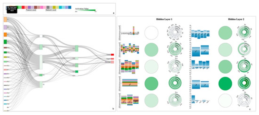
Figure 1. The proposed visual analytics to explain deep neural networks with neuron clustering. (a) A color-coded input feature layer along with feature descriptions. (b) Network level view: Represents a deep neural network to observe feature contribution to the predictions. (c) Feature level view: A detailed view of activation-based clustered neurons with a circular design and feature and neuron weights as a vertically stacked bar chart.
Visual analytics functions as a potent mechanism for decoding the underlying behaviors of deep learning systems [12]. Graphical interfaces can be leveraged to comprehend system architecture by mapping network elements like neurons and layers, to evaluate features by emphasizing how specific inputs drive predictions, and to compare system performance using standard evaluation metrics. Nonetheless, when processing high-dimensional data spaces and DNNs governed by extensive hyperparameters, visual analytics systems run into visual scalability bottlenecks that induce heavy visual clutter [13]. This clutter degrades visual interpretation and limits the information extracted from the graphics due to structural occlusion and general disorganization [14].
A substantial body of research has targeted the mitigation of visual clutter to deliver a more transparent perspective when visualizing deep neural networks. We categorize these investigations below according to their specific decluttering methodologies: filtering, reduction operations, edge bundling, and clustering, as detailed in Table 1. Investigators have frequently turned to filtering [15-18] to resolve visual clutter bottlenecks, as documented in Table 1. To illustrate, Deepvix [15] filters connection weights using a specific threshold limit applied to lines joining long short-term memory (LSTM) layers. Along similar lines, Summit [16] and ReVACNN [17] filter out network edges to thin down the visual clutter stemming from the sheer volume of channels and inter-layer links. GNNVis [18] deploys reduction operations to accelerate the rendering speeds of graph neural networks by filtering out peripheral nodes, thereby sharpening user focus. Filtering functions by displaying or highlighting targeted dimensions of the data while masking alternative elements. Be that as it may, this practice can introduce analytical bias depending on the filtering thresholds established by users or platform developers. Users and developers risk injecting bias by prioritizing isolated data components while disregarding others. Furthermore, filtering out weights, layers, or neurons can inadvertently purge outliers from the VA interface, stripping users of the chance to spot anomalous network characteristics.
To counteract the issues of analytical bias and overlooked outliers, dimensionality reduction (DR) strategies, such as t-distributed stochastic neighbor embedding (t-SNE) [19], have been widely integrated. For instance, Rauber et al. [20] harnessed dimensionality reduction workflows to map the activations across all hidden layers. DeepVID [21] employs t-SNE to display image structures within a scatterplot layout, enabling users to implement lasso selection tools to isolate data and audit the choices made by an NN. In a parallel fashion, ActiVis [7] incorporates t-SNE to aggregate subsets of instances matching their activation similarities. Within ActiVis [7], operators can isolate a specific cluster of instances on a projection display to evaluate them thoroughly. Even so, dimensionality reduction workflows face inherent limitations regarding the maximum volume of viewable points, particularly when handling the immense activation arrays of deep NNs [13]. Dimensionality reduction operations can still trigger graphical occlusions and overlapping data points, which can disorient users.
To overcome the limitations of DR approaches, Rauber et al. [20] incorporated a bundling algorithm [22] to augment the activation projection display by generating bundled layouts. Correspondingly, Cantareira et al. [23] implemented a related yet adapted bundling algorithm based on the work of Rauber et al. [20] to aggregate matching trajectories. Because edge bundling can still mask the explicit relationships within a given bundle—making it problematic to isolate individual integrated edges—Cantareira et al. [23] integrated control nodes into the algorithm to trace the pathways of activations across the training timeline.
More recently, clustering approaches have gained traction for rendering dense networks to circumvent screen real estate limitations and expose structural trends within massive graphs. As an example, Cakmak et al. [24] applied a hierarchical density-based spatial clustering technique [25] to diminish VC when mapping extended sequences of dynamic graphs. This clustering process grouped and structured related features inside pixel-centered visualizations to map temporal trends. Wu et al. [26] and Liu et al. [9] took advantage of k-means [27] to eliminate overlap when visualizing neuron activation patterns. In the same vein, Wongsuphasawat et al. [28] introduced a clustered network graph by organizing nodes according to their hierarchical arrangements, backing this up with an edge bundling algorithm. Liu et al. [5] engineered a visual analytics platform named CNNVis that blends both clustering and edge bundling models to yield an unobstructed perspective of training trends in convolutional neural networks (CNNs) structured as directed acyclic graphs. Clustering algorithms are capable of better preserving data points, neurons, and layers based on their internal similarities compared to filtering or sampling techniques [29]. Because many clustering methodologies demonstrate resilience against data noise and outliers, users can discover anomalous instances without suffering data loss. Additionally, clustering aids in data interpretation and clarifies core structural patterns.
Beyond standard decluttering frameworks, multiple tailored decluttering variants have emerged. For instance, Bellgardt et al. [30] leveraged immersive virtual reality (VR) to minimize visual clutter by introducing a third spatial dimension, rendering solely the edges tied to a user-selected node when mapping NNs as node-link diagrams. Ji et al. [31] created a dedicated platform, USEVis, optimized for attention-driven architectures, utilizing weight filters to strip away clutter and emphasize pivotal attention scores. Shen et al. [29] also engineered specialized sampling strips to suppress visual clutter when illustrating the classification outputs of DNNs.
Table 1. A comprehensive comparison between visual analytics tools.
Studies | Visual Clutter | Interactions | Purpose of Explanation | ||||
Filtering | Reduction Operations | Bundling | Clustering | Others | |||
Deepvix [15] | X | F, H, DM | AA, PA | ||||
Summit [16] | X | C, H | AA | ||||
ReVACNN [17] | X | F, DM | AA, PA | ||||
Rauber et al. [20] | X | X | C, F | FA | |||
CNNVis [8] | X | X | DM | AA, FA | |||
Wu et al. [26] | X | X | DM | PA, FA | |||
Activis [7] | X | DM | AA, FA | ||||
TensorFlow PlayGround [32] | A, DM | FA, PA | |||||
TensorBoard [33] | X | Node Expansion | C | AA, PA | |||
Bellgardt et al. [30] | X | 3D in VR | C | AA, PA | |||
DeepVID [21] | X | C | FA | ||||
USEVis [31] | X | Thresholds | C, F, DM | FA | |||
Shen et al. [29] | X | C, F | FA | ||||
Chae et al. [12] | Stripes design | C | FA, PA | ||||
Our VA tool | X | Circular design | C, H | AA, FA | |||
Interactions: H: Highlight, F: Filter, C: Controls, DM: Direct Manipulation, A: Animation. Explanation Type: AA: Architecture Analysis/Understanding, PA: Performance Analysis, FA: Feature Analysis/Selection.
Previous VA frameworks have mostly concentrated on thinning out visual crowding within CNNs [7, 8, 12, 16, 18, 21, 26] and recurrent neural networks (RNNs) [15, 29] because of their widespread adoption in computer vision and large language model domains, combined with their more intuitively interpretable structures. While CNN layouts are organized hierarchically to capture spatial configurations in visual media, RNNs incorporate recurrent loops tailored specifically for sequential data streams like audio files or text bodies. Conversely, although the overwhelming majority of practical corporate and scientific datasets are structured in tables, their matching deep learning variants—deep neural networks—are regularly sidelined in visualization and interpretability studies due to their sheer layer depth and massive neuron quantities. Furthermore, decoding a DNN is intrinsically harder because the network topology lacks inherent spatial or temporal constraints, making it highly difficult to trace how individual layers isolate and propagate data.
To address this technological gap, TensorBoard [33], designed by Google engineers, permits users to audit extensive NN structures through interactive zooming controls and node expansion options. This platform maps out a high-level conceptual schematic of the designer's model layout [33] rather than exposing the live internal parameters (such as weight updates or bias values). Because of this configuration, TensorBoard lacks any clustering mechanisms to consolidate layers or nodes for clutter suppression. In a similar vein, TensorFlow PlayGround [32] represents a popular environment built to let users interact with basic NN behaviors and adjust hyperparameters like layer counts and node capacities. However, this platform enforces a strict cap on the maximum number of hidden elements. Engineered primarily for pedagogy, it is limited to handling two abstract, real-valued input features [32]. It also completely overlooks decluttering controls, leading to heavy overlapping and legibility issues if users maximize layer or node counts.
Our work departs from these existing paradigms by focusing explicitly on unlocking the inner mechanics of deep, fully connected neural networks through direct graphical exposure of their parameter dynamics. Given the deficiencies of filtering—such as introducing analytical bias and erasing critical outliers or anomalous events—alongside the volume constraints that hamper dimensionality reduction methods [13], we chose clustering algorithms as our core engine to clean up intermediate layers and their components. Unlike TensorFlow PlayGround [32], our platform imposes no limits on network size or layer depth because our clustering method scales down visual density automatically. Additionally, our tool maps core parameters like weights and activation shifts directly. Practitioners can inspect any NN setup using this application without being constrained by layer or node maximums. Furthermore, while TensorFlow PlayGround [32] is optimized exclusively for two abstract features, our platform natively accommodates high-dimensional tabular matrices. We also deploy a distinctive circular design motif to display grouped neuron configurations compiled by activation similarities. These activation-grouped arrays allow users to seamlessly track information flows across consecutive network boundaries, making it much easier to comprehend how data propagates into final model predictions. By consolidating these variables into a compact visual display, we minimize cognitive fatigue and exploration times, allowing users to achieve a faster, clearer understanding of the underlying network.
Spurred by growing skepticism toward opaque models, the implementation of explainable artificial intelligence (XAI) models has risen rapidly [21, 34-36]. For example, DeepVID [21] leverages the Local Interpretable Model-Agnostic Explanations (LIME) [37] routine—a benchmark XAI method—to compute feature importance vectors, mapping these metrics directly onto images by highlighting localized pixels to explain individual NN decisions. Similarly, Wu et al. [26] integrated LIME within their visual framework to back instance-specific inquiries. XAI tools are typically limited to such instance-level analyses [21, 34, 36]. Most existing methodologies center on feature attribution [21, 34], isolating vital pixels through techniques like Saliency maps [38], Grad-CAM [39], or rule-based logic [40-42] that derive structured expressions using rule-extraction pipelines. These classic XAI models diagnose the behavioral outputs and prediction pathways of a DNN rather than illuminating the structural composition of the system itself [43]. While such attribution models yield useful clues about specific model behaviors, they cannot—unlike our proposed application—provide a comprehensive visualization of an NN's full layer configurations, individual nodes, and parameter vectors simultaneously. Our solution visualizes the network topography directly, incorporating averaged activation states through a tailored layout alongside multi-layer weight lines. By balancing comprehensive overviews (network-level view) with localized insights (feature-level view), we empower practitioners to audit and interpret complex NN behaviors effectively.
This section details the primary architectural difficulties encountered by ML developers and outlines the specific design targets established to overcome them within our system.
To build a highly effective interactive visual analytics environment for demystifying neural networks, we focused on three primary design challenges (DCs) highlighted across contemporary literature [7, 16, 43-45].
DC 1: Complex model architecture. Modern DNN frameworks consist of numerous hidden layers and hundreds of distinct nodes. Due to their opaque nature, the internal arithmetic, cross-layer operations, and prediction logic remain deeply hidden. Peeling back this layer of mystery requires exposing multiple network dimensions—ranging from high-level topology (layers, neurons) down to individual calculations (activation states)—showing explicitly how input attributes drive final classification scores, particularly for end-users or domain specialists unfamiliar with advanced ML.
DC 2: Visual clutter and scalability. Graphically rendering modern NNs creates immediate visual crowding and scaling roadblocks due to the sheer density of components. Squeezing massive layer arrays, dense connection vectors, and secondary numerical attributes like weights into a fixed screen space compromises human visual perception. Constructing a scalable visualization requires a careful trade-off between dropping unnecessary visual noise and preserving vital informational structures.
DC 3: Underrepresented data domains. While current VA platforms regularly rely on image or text inputs to explain DNN operations [1, 6-8], tabular formats remain heavily neglected, despite forming the backbone of most industrial data applications. Moreover, working with tabular records introduces extra visualization challenges, such as representing learned features, managing mismatched data types, and handling sparse or missing values.
In response to these challenges, we defined our underlying design goals (DGs) as follows:
DG 1: Presenting a compact architecture view by reducing the clutter. Structuring data within a streamlined layout prevents user cognitive exhaustion. Because DNN systems are characterized by vast layer depths and high node counts (DC 1), we aim to establish a consolidated interface displaying layers and neurons where an automated clustering routine handles the suppression of node clutter (DC 2).
DG 2: Interpret tabular data features in NN decision. Interpreting tabular layouts is significantly harder than analyzing image profiles, which are inherently intuitive. We intend to use a tabular dataset as our primary validation use case (DC 3), focusing on how structural features feed into individual neurons and ultimately shape classification outcomes through interactive visual elements.
For our experimental evaluation, we employed the Cardiotocography (CTG) dataset obtained from the UCI Machine Learning repository [46]. Cardiotocography serves as a clinical technique to assess fetal well-being by monitoring the baby's fetal heart rate (FHR) concurrently with maternal uterine contractions during pregnancy [47]. This specific dataset is gathered via the SisPorto system [48], which processes digital signals captured from a fetal monitor. Obstetricians analyze CTGs by interpreting FHR trends. Generating precise diagnoses and distinguishing between normal and abnormal physiological trends is vital to mitigate the risks of conditions like cerebral palsy and neurodevelopmental disabilities [49].
To minimize clinical workload and diagnostic subjectivity when evaluating CTGs, machine learning models are routinely introduced as decision-support systems. The dataset comprises 2126 fetal CTG observations spanning 21 features derived from the underlying cardiotocographic waveforms. These records were manually categorized by three professional obstetricians to assign a consensus classification label to each case. Analytical tasks can be executed using either the 10-class morphologic pattern classification or the 3-class fetal state classification. In terms of distribution, the dataset consists of 1655 observations designated as normal, 295 observations labeled as suspect, and 176 observations categorized as pathologic.
The data pipeline encompassed data cleaning, training-testing partitioning, and cross-validation phases. Hyperparameter tuning via grid search led to the selection of the rectified linear unit (ReLU) activation function combined with the Adam optimizer. The learning rate configuration was set to adaptive. To eliminate selection bias, a 10-fold cross-validation scheme was implemented, randomly partitioning the data into 80% for model training and 20% for testing. Following empirical validation and grid search optimization, a 4-layer NN architecture was chosen based on predictive accuracy. This selected NN framework incorporates hidden layers configured with 30 and 20 neurons, respectively, yielding an optimal accuracy score of 0.88. The computational pipeline was implemented using Python, while all interactive visual modules were constructed via the D3 [50] JavaScript library.
When clarifying the internal predictive logic of an NN, researchers often focus on tracking how individual neuron activation states fluctuate over the course of training. Activation functions drive the transmission of information across subsequent layers, with elevated activation magnitudes generally signifying heightened neural engagement. Against this backdrop, we introduce a methodology designed to extract and isolate the activation values for every individual neuron. Because the total count of hidden neurons and corresponding activations can scale drastically into the hundreds or thousands, we propose computing the average activation value per neuron across each target class to resolve the challenges of high dimensionality.
Suppose we establish an activation matrix A, as mapped out in Figure 2, where columns nj denote the jth hidden neuron within a given layer, rows tik reflect the training instances associated with class k (ck), and entries aij represent the specific activation value elicited by the ith training instance at the jth neuron. The baseline activation matrix A possesses dimensions of I·J , where I represents the total quantity of training instances and J denotes the number of hidden units within the structural layers. To condense the dimensionality of this activation space, we isolate a subset T of training instances belonging exclusively to class ck. For any target class ck, Tk defines the set of index values tracking the training records that fall under class ck. To illustrate:
Following this partitioning, we compute the arithmetic mean of each activation cohort per class to extract a single consolidated activation value using the following structural relationship.
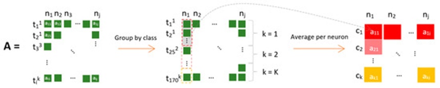
Figure 2. Obtaining the average activation values per neuron at each class. The activation matrix (A) is grouped by class per neuron (nj) and each class (ck) has an averaged activation value (aij).
Consequently, we derive a updated, averaged activation matrix for our subsequent clustering experiments, yielding a reduced dimension of Ak·j, where k represents the number of target classes in the dataset. This compressed matrix provides a concise representation of network activations by downscaling the spatial dimensions from the baseline I·J framework to a compact K·J matrix. By introducing this neuron clustering paradigm, we intend to alleviate the visual clutter hampering node and link layouts by consolidating related neurons into macro-level "mega neurons."
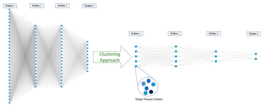
Figure 3. demonstrates an operational example of minimizing visual clutter across both node representations and connection pathways by generating mega clusters within a 4-layer NN framework. This mega-neuron architecture aims to lower visual density while simultaneously categorizing neurons that exhibit correlated operational patterns. Users can examine and evaluate these mega-neurons to diagnose collective hidden activation trends, such as identifying highly reactive node groups versus dead neurons, converting an entire group of clustered units into a single mega cluster reflecting equivalent activation behaviors.
We tested a variety of clustering frameworks to group hidden units based on similarity profiles derived from the averaged activation matrix, including k-means [27], mean shift [51], and hierarchical clustering [52]. The mean shift routine operates without requiring a predefined cluster count, whereas the ideal cluster counts for k-means and hierarchical configurations were derived through empirical testing. For the k-means algorithm, cluster counts were assessed by computing the sum of squared distances between cluster centroids and their respective data members, denoted as the sum of squared errors (SSE). Figure 4a demonstrates the selection process for the optimal cluster count within the first hidden layer utilizing the elbow method. The elbow approach aids in identifying the ideal cluster count by pinpointing the inflection point along the plotted SSE trajectory line. Conversely, a dendrogram utilizing the Ward distance metric [53] was employed to isolate the cluster counts for the hierarchical model. Figure 4b maps out the first hidden layer's dendrogram alongside its Ward distance values and resulting clusters, where tree height indicates inter-cluster distance. Through this hierarchical tree, the cluster count for the first hidden layer was established at four. For the k-means model, the first hidden layer cluster count was fixed at five based on the corresponding SSE metrics.
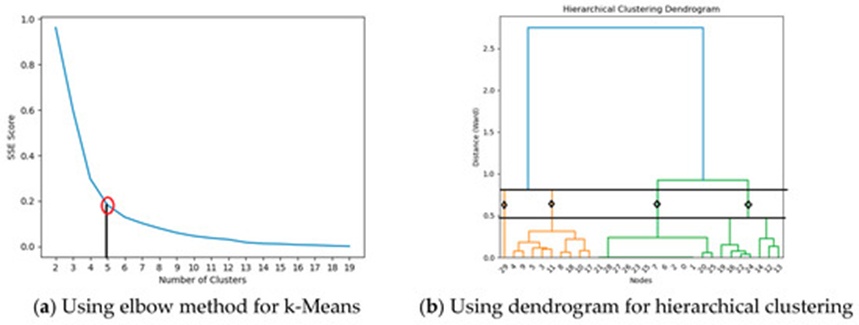
Figure 4. The selection of a number of clusters for k-means (a) and hierarchical clustering (b).
Given that the ground-truth cluster labels for hidden neurons are inherently unavailable, we evaluated our configurations using the Silhouette, Davies-Bouldin (DB), and Calinski-Harabasz (CH) validation metrics [54]. The resulting clustering outputs, the cluster counts for the second hidden layer, and the matching validation metrics are detailed in Table 2.
Table 2. The comparison of neuron clustering results is based on evaluation metrics.
Hidden Layer | Clustering Technique | Highest CH Score | Lowest DB Score | Highest Silhouette Score | Cluster Count |
First Hidden Layer | K-means | 159.44 | 0.49 | 0.632 | 5 |
First Hidden Layer | Mean Shift | 143.28 | 0.40 | 0.60 | 6 |
First Hidden Layer | Hierarchical Clustering | 131.76 | 0.46 | 0.630 | 4 |
Second Hidden Layer | K-means | 41.60 | 0.53 | 0.59 | 5 |
Second Hidden Layer | Mean Shift | 36.03 | 0.47 | 0.58 | 4 |
Second Hidden Layer | Hierarchical Clustering | 28.50 | 0.60 | 0.56 | 4 |
Note: The optimal performance scores are highlighted in bold within the layout. The empirical trends documented in Table 2 reveal that the mean shift and k-means models surpassed the hierarchical clustering workflows when grouping hidden units across both structural layers. Hierarchical clustering yielded depressed performance on the Silhouette and CH benchmarks—where higher scores denote superior separation—whereas k-means secured the top scores on these indicators for both hidden layers. Correspondingly, mean shift achieved the strongest DB marks, which optimize at a minimum value, while the hierarchical model performed poorly on the DB framework. Although the mean shift method demonstrated a stronger DB score relative to k-means and hierarchical clustering, a deeper evaluation of its output distribution showed that an overwhelming majority of neurons were funneled into a single massive group. The high internal variance of activation attributes across these groups demonstrates that mean shift fails to properly represent identically behaving neurons.
As a result, we omitted the mean shift algorithm from our interactive interface. In the same manner, the hierarchical clustering approach was discarded due to its weak performance profile across the DB and CH metrics. We ultimately integrated the k-means algorithm into our visualization architecture based on these performance metrics, as it consistently led across at least two validation benchmarks for each hidden layer. Guided by the elbow method, we deployed five clusters (mega neurons) via k-means for each hidden layer within the network.
We structured our visualization environment to feature distinct feature-level and network-level interfaces, supporting both comprehensive macro-examinations and localized micro-examinations. The network-level display integrates a Sankey diagram (Figure 5a) representing the comprehensive NN layout via consolidated mega-neurons. The links mapping connections between the Sankey nodes correspond to the underlying model weights driving the layers, where link width scales proportionally with weight magnitude. This Sankey configuration lets users instantly assess relative weight balances among neuron groups while tracking broader network properties, such as weight distributions flowing from the input layer to the final prediction output.
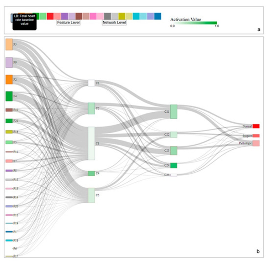
Figure 5. A compact view of neural networks with clustered mega neurons. (a) represents the legend of input layer along with feature definitions and a color legend for activations. (b) Sankey diagram represents network level visualization.
Each individual metric within the dataset is designated as F#, where the symbol # denotes the specific index of that attribute within the CTG database. Comprehensive clarifications regarding this feature collection are accessible via the UCI ML repository [46]. Because link thickness reflects weight magnitude—such as with attribute 6 in the primary input tier—F6 (representing severe decelerations per second) exhibits the faintest links to the initial hidden tier, illustrating that F6 yields a minor impact on model forecasts. Conversely, stronger linkages to the first hidden tier are observed for F2 (accelerations per second), F3 (fetal movements per second), F4 (uterine contractions per second), and F9 (the average value of short-term variability). These specific attributes provide a more substantial impact on the forecasts generated by the model, as corroborated by [55].
Monitoring uterine contractions (F4) remains critical throughout gestation to track both fetal and maternal health. Comparable observations have been documented across established literature [55].
The Sankey illustration is constructed utilizing a breadth-first search approach. To enable domain specialists and end-users to adjust the sequence of the input tier and aggregate elements according to weight magnitudes, the nodes within the Sankey illustrations can be rearranged via dragging (Figure 6).
Because the instrument was engineered specifically for tabular data structures, input data attributes are integrated as shaded indicators featuring definitions embedded within a hover tooltip (Figure 5b). The initial input tier applies categorical shading where each hue denotes a distinct data attribute, as displayed in the primary tier of the Sankey illustration (Figure 5a). The color intensity exhibited on each mega neuron—displayed as rectangular units in the Sankey illustration—reflects the scale of neural activity occurring within that specific group. The color scale for these activations ranges from white to green depending on magnitude; white signifies the minimal activation level, whereas green points to the maximum level of activation (Figure 5a). Shading density on the final output tier corresponds directly to the volume of instances within each respective category. As an illustration, the normal category encompasses 1655 instances and is highlighted in a vivid red tone, whereas the pathologic category contains 176 instances and is marked by the faintest red shade. Alongside analyzing the core framework, users can evaluate dataset characteristics regarding attribute weights by tracking the linkages spanning across tiers and reviewing the volume of the final output categories.
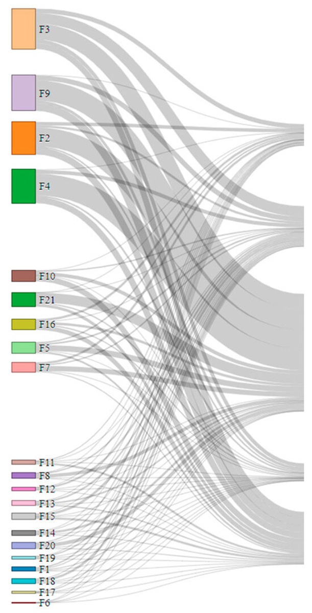
Figure 6. An example of an input layer grouped based on their contributions to the prediction with a drag and drop option. F3, F9, F2 and F4 have the highest weights as supported in literature [55].
Operators can transition to the attribute-specific perspective by interacting with the 'feature level' toggle positioned on the input tier explanation legend. This attribute-specific perspective (Figure 7) delivers an explicit breakdown of attribute weights for individual neurons inside each respective group. These attribute weights are displayed using a stacked vertical bar chart (Figure 7a) that incorporates attribute-specific shading for each group. The vertical axis measures the weight values of every attribute per neuron, whereas the horizontal axis maps out the corresponding neurons contained within each mega neuron. The height of every individual block reflects its weight value, spanning both positive and negative directions based on its alignment along the vertical axis. A secondary stacked vertical bar chart illustrates the weights operating between consecutive hidden tiers, where the color indicates the overall scale of these weights.
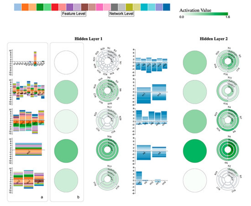
Figure 7. A feature level view of the proposed visualization tool. Feature level shows a stacked bar chart to represent weights, circular mega neurons, and a circular custom design to show each neuron within clusters with activation values. (a) Vertical stacked bar chart for feature weights. Colors indicate individual features, as seen in legend. (b) Mega neurons that represent clustered neurons based on averaged activations. Mega neurons are colored based on their average activation value as shown in legend.
Operating on the outcomes of k-means clustering, five distinct groups are established at each hidden tier. Users can open the expanded perspective of mega neurons, as displayed in Figure 7b, by selecting any mega group to open a specialized circular layout. This attribute-specific perspective maps out the training behavior (encompassing weights and activations) along with the inner representations of the intermediate tier.
Figure 8 displays the expanded perspective of group 1 situated within the initial hidden tier. This targeted view incorporates a specialized layout engineered to isolate and display every individual neuron residing in a group. The concentric circular rings indicate the aggregate quantity of target categories. Given that the CTG dataset features three distinct categories, the grouped neuron layout comprises 3-layered concentric circles (Figure 8), representing the normal, suspect, and pathologic categories. The applied color reflects the span of activation values. Although the mega neuron initially presents a white shade—denoting near-zero activation levels—interacting with it opens an expanded perspective for evaluating every separate neuron by highlighting and inspecting granular data via the hover tooltip. Validated by the attribute weights, it is apparent that highlighted neuron 26 holds an activation value of 0.117 for the pathologic category, whereas the remaining neurons exhibit zero activation, signifying that they do not forward information to subsequent tiers and remain non-contributory to the optimization process.
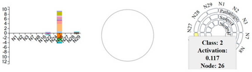
Figure 8. Mega neuron 1 at the first hidden layer, along with feature weights. The color legend indicates that most of the neurons at cluster 1 are not activated (dead).
Figure 9 provides a comparative evaluation between mega neurons (groups) 4 and 5 across both hidden tiers. As illustrated in Figure 9a, group 4 within the initial hidden tier contains a solitary neuron (neuron 30), whereas it holds two neurons (neurons 9 and 6) inside the subsequent hidden tier. High-activation neurons are present across both tiers, exemplified by neuron 6 of the normal category, which reaches an activation value of 1.574. This indicates that N30 can successfully transmit information to subsequent tiers through elevated activation values, contributing meaningfully to final forecasts. As revealed by the stacked bar chart, F2, F3, F4, and F4 (tracking the color key) display elevated weights relative to alternative attributes. Conversely, group 5 (Figure 9b) encompasses three neurons in hidden tier 1 and five neurons in hidden tier 2. Group 5 displays moderately lower activation levels relative to Group 4, with the scale of activation diminishing further at the secondary hidden tier. For instance, the activation value recorded for neuron 2 within the pathologic category stands at 0.295. It can be seen that comparable color densities aggregate together, demonstrating that the clustering routine successfully isolated and categorized equivalent activation behaviors. Interaction features like highlighting, zooming in, and zooming out are integrated into the design to augment user engagement, enabling operators to either review the macro-level layout or isolate specific micro-level details.
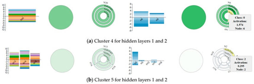
Figure 9. Clusters 4 and 5 for both hidden layers, along with the weights. Cluster 4 has highly activated neurons while cluster 5 at the second hidden layer is almost zero.
We introduced a visualization platform that implements a clustering routine, specifically k-means, alongside a distinctive circular layout to mitigate visual clutter. Following a grid search optimization for NN hyperparameters and empirical testing to establish the ideal count of hidden tiers and neurons, we selected the top-performing framework. This framework consists of an input tier containing 21 attributes (nodes), two hidden tiers containing 30 and 20 neurons respectively, and an output tier containing 3 target categories (nodes). The aggregate node count in this chosen framework equals 74, connected by 1290 interlocking edges between tiers. Through the deployment of k-means, the quantity of hidden neurons was condensed from 30 and 20 down to 5 mega neurons. Consequently, the total node count dropped from 74 to 34, marking a 54% reduction, which implicitly lowered the total number of inter-tier edges from 1290 down to 145, representing an 88.7% contraction. While the system displays aggregated mega neurons, it simultaneously empowers users to drill down into the granular configurations of individual neurons via a specialized layout that minimizes visual complexity. This approach circumvents the processing drawbacks of alternative data-aggregation strategies—such as data omission—by preserving the authentic hidden neurons alongside their precise activation values. This combined macro and micro perspective assists users in deciphering the underlying behavior of NNs by allowing them to trace how data propagates through network weights. Color-coded mega neurons further streamline the evaluation of active versus inactive (dead) neurons that guide the network's predictive processing. Recognizing these inactive neurons allows machine learning engineers to refine their network configurations by scaling down unnecessary units. The analytical breakdown is organized into three distinct sub-sections: scalability and visual clutter, the performance efficacy of the platform, and its current constraints.
Scalability and clutter: This research prioritizes the reduction of visual clutter across neuron representations within neural network visualization models. To visually clarify deep neural networks, we targeted a pervasive challenge within the visual analytics discipline: visual clutter. Clustering techniques were leveraged to categorize neurons according to similarities in their calculated activation values. A tabular medical dataset was used to optimize the deep neural network and verify its internal components through a real-world use-case scenario. Activation values were gathered post-training to formulate an averaged activation matrix by computing mean activation parameters for every category. This aggregated matrix mitigates the challenges linked to high-dimensional datasets by consolidating activations at a category-specific tier. We assessed three widely implemented clustering techniques—k-means, mean-shift, and hierarchical clustering—for integration into the application. This evaluation relied on three performance benchmarks: the Silhouette score, the Davies Bouldin index, and the Calinski Harabasz index. Based on these evaluations, the hierarchical clustering technique failed to deliver viable outcomes, whereas k-means outpaced alternative clustering methods across at least two performance benchmarks. The optimal cluster count for each hidden tier was set at five using the elbow selection method. The benchmarks proved that k-means successfully organized the neurons by gathering them based on activation profile uniformities. These groups were mapped out as mega neurons that encapsulate every internal neuron of the cluster. Representing data via mega neurons successfully alleviated visual density across each hidden tier. Compressing the neuron volume into compact mega neurons simultaneously minimized edge intersection clutter spanning between tiers. Users can access the granular details of these mega neurons via interactive toggles. This specialized grouped-neuron layout presents all relevant information within a compact space without over-saturating the operator. The applied color density enables users to easily trace highly active pathways alongside dead neurons that remain non-contributory to the learning process. Additionally, input attributes are displayed as color-coded indicators that feature standalone explanations via hover tooltips.
Efficacy: This study utilizes a tabular healthcare dataset to execute an operational use-case scenario. The objective is to map out activation values during the training phase to show how data transfers from tier to tier. Following model optimization, network weights and adjacent computational variables (such as activations) were pulled from the system. The resulting layout highlights the fluctuations of activation profiles across various neurons. Operators can distinguish between active and idle neurons at every individual tier via color density variations. It was noted that the initial hidden tier contains a higher concentration of idle neurons relative to the secondary tier. Furthermore, group 4 within the secondary hidden tier exhibits higher overall activation values. This observation confirms that successive tiers isolate and interpret increasingly intricate attributes to formulate the final output. As a result, the impact of neurons in the secondary tier on the final output tier is more pronounced. The layout yields clear insights regarding the internal activations of neural networks. The system structure adheres to foundational visual design paradigms: macro-overview first, zooming and filtering actions, followed by detail-on-demand features. This use-case scenario demonstrates system efficacy by breaking down the core elements of a neural network trained on tabular data records. The overall architecture is presented first at a macro level. Following this, interactive controls are utilized to extract detail-on-demand views detailing separate activations and attribute weights. This strategy minimizes visual overcrowding via a clustering routine and an original circular layout, assisting in demystifying black-box models. Within the attribute-level perspective, feature weights are presented as a color-coded, vertically stacked bar chart linking the input tier to the initial hidden tier, along with an equivalent layout mapping the weights between the first and second hidden tiers. Users can immediately pinpoint the attributes yielding the highest impact on forecasts by observing the heights of the bar chart elements. These interpretations are further corroborated by matching studies [40] centered within the clinical data space.
Limitations: The introduced layout was created for domain specialists and end-users to clarify the operational tendencies of neural networks using both network-wide and feature-specific interfaces. The design facilitates the visual tracking of internal network parameters, namely weights and activation values. However, auxiliary computational metrics—such as gradients and parameter deltas—could be incorporated to further assist data scientists and machine learning specialists in deciphering network models. Although minimizing neuron and edge intersection density via clustering techniques serves as the primary innovation, incorporating an edge bundling technique would address the current issue of overlapping link paths. An additional constraint centers on the fact that this visualization instrument was verified solely through a single use-case study in the clinical medicine sector. To counter this constraint, subsequent research will focus on structuring user evaluation studies to increase the empirical validation of the instrument. These user studies will gather qualitative feedback on software usability, verify efficiency regarding user insights, and refine the visualization layout according to user specifications and testing feedback. The current use-case model involves a limited feature set that is straightforward to display at the input tier. As dataset dimensionality scales up, managing massive feature volumes without generating visual clutter becomes difficult. Consequently, operators may require options to isolate only the most critical attributes. This limitation can be managed in future iterations by embedding feature selection and attribute importance methodologies directly into the existing interface. Expanding the interactive options—such as introducing direct manipulation features—will similarly resolve current limits regarding real-time parameter tuning.
We presented a visual layout designed to improve the explainability of neural networks through their core computational variables. Clustering models were deployed to categorize hidden neurons based on activation profile uniformities to manage visual clutter, a frequent issue encountered when mapping out NN architectures. We introduced mega neurons to signify clustered neurons utilizing the top-performing clustering approach, namely k-means. Mapping out the neural network framework through these condensed mega neurons effectively neutralized visual overcrowding. To let users drill down into the specific activation profiles of individual neurons, interactive options were built into the software. This configuration enables the evaluation of neurons according to their functional status: active or idle. We also determined that downstream tiers provide a more substantial contribution to final forecasts because they systematically isolate more intricate data characteristics. Utilizing a color-coded feature weight visualization layout enabled the identification of high-importance attributes. These outcomes align with and are validated by existing research.
Subsequent research efforts will target the resolution of these system constraints to upgrade the interface and display a broader array of neural network variables. We will prioritize the integration of additional variables, specifically gradients and attribute importance metrics. Future developments will also seek to expand interactive features and permit direct adjustments so operators can alter parameters and observe immediate shifts in model forecasts. Integrating direct manipulation will also assist users in isolating the attributes that yield the highest impact. Operators could systematically eliminate features one by one until a shift occurs in the categorical prediction. The developed visualization instrument will be rigorously tested against highly complex, high-dimensional tabular datasets and deep neural network models to verify its functional scalability. Moving forward, we also intend to set up user evaluation studies involving machine learning engineers and domain specialists to optimize the layout, enhance operational features, and collect feedback regarding platform usability. Furthermore, upcoming initiatives will focus on embedding advanced artificial intelligence systems within the VA framework to explain these black-box operations both mathematically and visually.
None
None
None
None
Open Access The author(s) retain copyright. This article is licensed under the Creative Commons Attribution-NonCommercial-ShareAlike 4.0 International License. It may be shared and adapted for non-commercial purposes with appropriate attribution, an indication of changes, and distribution of adaptations under the same license. Third-party material may be subject to separate terms identified in its credit line. View the license at https://creativecommons.org/licenses/by-nc-sa/4.0/.
 Transparent Intelligence Publishing