Equatorial plasma bubbles (EPBs) represent areas of reduced electron density that develop within Earth’s ionosphere as a result of Rayleigh–Taylor instability. These formations can trigger signal scintillation, which induces signal degradation and navigation positioning inaccuracies. EPBs can be identified via imagery gathered by All-Sky Imager (ASI) networks. The present research introduces an inexpensive, automated technique for identifying EPBs within ASI datasets, suitable for real-time monitoring as well as categorization tasks. This approach couples Two-Dimensional Principal Component Analysis (2DPCA) and Recursive Feature Elimination (RFE) alongside a Random Forest machine learning classifier to construct an Explainable Artificial Intelligence (XAI) framework. This framework extracts image characteristics to automate EPB detection using minimal dimensionality, yielding a compact and exceptionally rapid-to-train model designed to discern EPBs in recorded ASI frames. A collection of 2458 images, categorized into "Event" and "Empty" classes, was assembled to construct the database. This image repository was partitioned randomly into two distinct portions: an 80% training dataset and a 20% testing dataset. The developed XAI framework achieved a marginally better detection accuracy relative to the conventional 2DPCA approach while maintaining a notably smaller structural footprint. Additionally, the execution of the proposed framework was assessed and contrasted against alternative deep learning baselines (ResNet18, Inception-V3, VGG16, and VGG19) under identical environmental conditions.
Equatorial plasma bubbles (EPBs) are frequently observed phenomena during nighttime in the low-latitude ionospheric F region, distinguished by sharp, abrupt drops in plasma local density [1]. The Rayleigh–Taylor instability is widely accepted as the primary driving mechanism behind the generation of these plasma structures [2]. These bubbles induce substantial scintillation of radio signals emitted from orbital satellites, and the resulting ionospheric turbulence can badly disrupt telecommunication and navigational infrastructures, including the Global Navigation Satellite System (GNSS). Consequently, this induces propagation delays and a generalized decline in system reliability [3–6]. Data gathered from optical instruments and satellite observations indicate that EPBs are magnetic-field-aligned structural bands characterized by depleted ionospheric plasma density that is notably lower than the ambient background medium [7–10].
As these plasma perturbations rise to higher altitudes, they map poleward along prevailing magnetic field lines, manifesting as localized drops in optical airglow intensity (OI 630.0 nm) within nightglow observations. These distinct dark bands are conventionally recognized as equatorial plasma bubbles (EPBs) [11]. This specific OI 630.0 nm emission, which is recordable via CCD imaging sensors, takes place in the lower F layer (250-300 km) and is driven by the dissociative recombination of O_{2}^{+} with ambient electrons according to the underlying pathways:
 (1)
 (2)
 (3)
where O(1D) denotes a metastable excited state [12, 13].
A substantial body of literature has leveraged optical sensors and CCD arrays to record images of equatorial plasma bubbles (EPBs) [10, 14–27]. For instance, Gentile et al. [28] executed an investigation leveraging plasma density observations gathered from DMSP to detect EPBs relative to ambient plasma backgrounds and compute occurrence frequencies across global orbits from 1989 through 2004. Similarly, Huang and Roddy [29] analyzed ion density observations collected by C/NOFS spanning 2008 to 2014 to map EPB events. Wan et al. [30] processed Swarm electron density profiles to detect and analyze the structural development of EPBs. Adkins and England [31] turned to 135.6 nm far-ultraviolet data provided by the Global-scale Observations of the Limb and Disk (GOLD) instrument to establish a technique for the automated identification and tracking of EPBs. Finally, Chakrabarti et al. [32] pioneered a deep learning methodology to precisely track the occurrence of plasma bubbles within ASI imagery.
Two-dimensional principal component analysis (2DPCA) has frequently been implemented to downscale data dimensionality while safeguarding vital spatial configurations, thereby boosting feature extraction and target classification performance [33]. This approach has been deployed across various disciplines for detection and recognition operations because it bypasses vectorization by directly evaluating two-dimensional data matrices. Lin [34, 35] and Lin et al. [36] applied 2DPCA to map anomalies in ionospheric total electron content (TEC) occurring prior to seismic events across diverse geographic zones. Yu and Liu [37] engineered a convolutional autoencoder founded on 2DPCA concepts specialized for classifying faults in wafer maps. Within computer vision frameworks, Sun et al. [38] presented a randomized nonlinear 2DPCA framework tailored for object identification by combining 2DPCA operations with random Fourier feature maps and non-linear activation functions. Furthermore, it has been integrated within bioinformatics alongside Rotation Forest strategies to predict protein–protein interactions [39] and implemented to forecast genetic mutations linked to lung cancer [40]. Such varied research implementations highlight the adaptive nature and utility of 2DPCA for evaluating two-dimensional matrix configurations across diverse monitoring environments.
Explainable Artificial Intelligence (XAI) incorporates various methodologies that primarily diverge into two strategies: post hoc and ante hoc frameworks. Post hoc interpretability metrics, including SHAP [41] and LIME [42], generate explanations after model training concludes. Though highly adaptable, their surrogate nature can occasionally diminish their perceived reliability in critical operations. By contrast, ante hoc strategies embed interpretability directly into the architectural layout of the model, yielding intrinsic transparency at the expense of potential constraints on operational flexibility and structural complexity. Research by Retzlaff et al. [43] delivers relevant oversight on this topic, offering design paradigms that clarify the functional variations and operational roles of post hoc versus ante hoc frameworks. Their work underscores that post hoc diagnostic tools are optimized for complex black-box configurations that demand independent explanation layers, whereas ante hoc solutions are superior in contexts where interpretable processing paths are a mandatory baseline from the design phase [43]. Comprehending these core distinctions is essential for connecting theoretical breakthroughs with practical deployments in XAI fields.
In this work, we present an alternative framework for the automated identification of EPB signatures in ASI observations utilizing an ante hoc XAI structure. This setup relies on Two-Dimensional Principal Component Analysis (2DPCA) coupled with Recursive Feature Elimination (RFE) paired with a Random Forest model. The presented approach demands dramatically lower computational resources and functions under far simpler hardware requirements. Moreover, it achieves extremely short training durations relative to deep learning configurations operating in identical environments, thereby streamlining the sorting of historical archives and empowering real-time detection of ionospheric plasma bubbles on inexpensive computing platforms.
Prior to compiling the diagnostic database, the raw frames were subjected to an initial preprocessing routine. To boost the visible structural components within the photographs and ensure the accurate selection of images for each dataset tier, a histogram equalization technique [44] was implemented using the following protocol:
 (4)
First, determine the image histogram via Eq. 4. The frame encompasses individual pixel intensities varying from r = 0, indicating the darkest boundary value, to r = L - 1, representing the brightest possible value, where L defines the cumulative sum of available intensity steps:
where k denotes the specific intensity tier, nk is the total count of pixels holding an intensity of rk, and n represents the total pixel count of the processed image.
Next, calculate the Cumulative Distribution Function (CDF) utilizing the expression below:
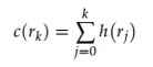 (5)
Conclusively, implement the mapping function to derive the adjusted pixel intensities via Eq. 6:
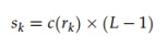 (6)
where sk signifies the transformed pixel intensity step and L denotes the total number of possible intensity levels.
Figure 1a displays an illustrative raw frame acquired at the Bom Jesus da Lapa (BJL) monitoring post (Geo 13.3 °S, 43.5 °W) on 8 October 2021 at 00:02:25. The corresponding pixel histogram for this frame is outlined in Figure 1b, demonstrating that the vast majority of pixel brightness tiers are grouped toward the darker boundary of the plot. Conversely, Figure 1c presents the identical image frame following contrast optimization, revealing hidden features via the outlined equalizing routine. The resulting histogram for this modified image is illustrated in Figure 1d, which reveals that pixel values are now dispersed across the entire operational scale, thereby maximizing visual clarity.
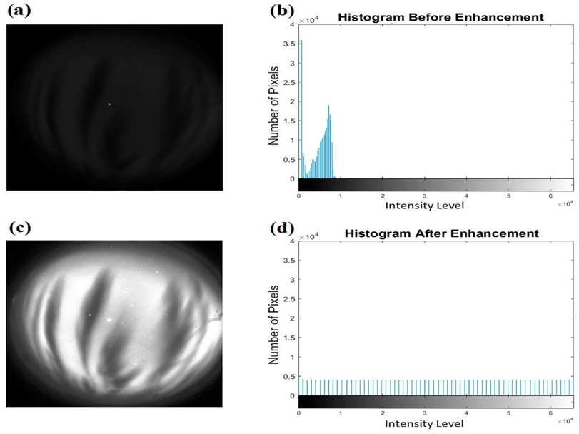
Figure 1. Raw frame from the BJL monitoring post (a) accompanied by its respective pixel histogram (b), whereas (c) illustrates the identical frame following contrast optimization and (d) displays the equalized histogram.
The ASI data utilized in this investigation were gathered from the BJL (Geo 13.3◦S, 43.5◦W) and São João do Cariri (CA) (Geo 7.4◦S, 36.6◦W) observatories. These observation stations are components of the Embrace/INPE network. The data acquisition timeframe extends from January 2020 to January 2022. Local time and seasonal variations were accounted for during dataset compilation. The collection comprises 2458 raw ASI images, which were manually categorized using their corresponding contrast-enhanced versions. The dataset was partitioned into two distinct classes. The first is the ‘Event’ Class, which encompasses images displaying observable plasma bubbles characterized by clear reductions in brightness and elongated topologies aligned with Earth’s magnetic field lines, originating at the magnetic equator and extending poleward, as illustrated in Figure 2. The second is the ‘Empty’ Class, which consists of images devoid of discernable plasma bubble structures. The first class contains 1242 images, whereas the second contains 1216 images. This database was subsequently partitioned randomly into two subsets: a training set and a testing set, adhering to a split of 80% for training (1967 images) and 20% for testing (491 images). This distribution ensures an adequate volume of samples for model training while retaining a sufficient quantity for testing evaluation.
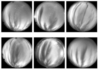
Figure 2. Visual examples of the detected EPBs.
To optimize the detection workflow, the designated datasets were converted using the Radon transform. The Radon transform is a mathematical operation that maps a two-dimensional spatial function (image) f(x, y) into a collection of its projections, with the origin x = 0 and y = 0 positioned at the geometric center of the image. The generated projection represents the integrated sum of pixel intensities along specified paths, effectively establishing line integrals evaluated across multiple orientations. This operation yields a modified image space designated as R(ρ, θ) [45].
(7)
where \rho denotes the perpendicular distance from the coordinate origin to the line, and \theta represents the angle formed between the line's normal vector and the horizontal x-axis. The mechanics of this transformation process are illustrated in Figure 3.
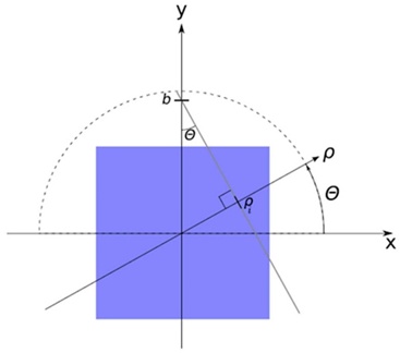
Figure 3. The summation line is given by the equation y = ax + b. Using trigonometry, the inclination a is found to be a = − and the intersection with the y axis is b = . This aligns with Eq. 4. These parameters are calculated for each combination of \theta and \rho. The maximum \rho is set to the length of the image’s diagonal line [45].
Mathematically, the Radon transform is formulated via the following expressions:
 (8)
where δ signifies the Dirac delta function.
Figure 4 displays instances of the primary images f(x, y) with dimensions of 512 \times 512 pixels alongside their respective Radon-transformed representations R(ρ, θ) possessing dimensions of 729 \times 180 pixels for exemplars from both classes. Figure 4a depicts the original image belonging to the “Empty” class, while Figure 4b illustrates its corresponding Radon-transformed profile. Similarly, Figure 4c shows the original image belonging to the “Event” class, and Figure 4d displays its transformed variant.
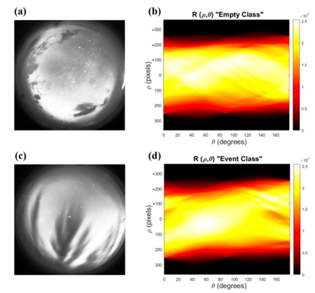
Figure 4. Example of original images f(x, y) and their corresponding Radon-transformed images R(\rho, \theta) for samples from each class: (a) Original image of the “Empty” class, (b) Transformed image of the “Empty” class, (c) Original image of the “Event” class, (d) Transformed image of the “Event” class.
The foundational principle of Two-Dimensional Principal Component Analysis (2DPCA) centers on deriving an m-dimensional projected vector capturing the essential features of an image through the following linear mapping operation:
(9)
where A represents an image matrix of size m \times n, X denotes a unitary column vector, and Y signifies the projected feature vector corresponding to image A [33]. For the raw airglow imagery (Figure 4c) acquired at the BJL station, the dimensions of matrix A are 512 \times 512. Meanwhile, for the Radon-transformed imagery (Figure 4d), the dimensions of matrix A are 729 \times 180.
The procedure begins by constructing a non-negative definite n \times n matrix designated as the image covariance matrix Gt using the designated training dataset:
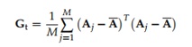 (10)
where M denotes the total count of training image samples, Aj represents the jth image matrix within the training dataset, and \bar{A} is the mean image matrix computed across all training images.
To identify an effective projection vector X, its descriptive capacity is quantified utilizing the total scatter of the projected instances. The trace of the covariance matrix derived from the projected feature vectors serves to define this total scatter. A larger trace value points to an optimized projection vector, as it signifies increased variance and enhanced separation among the projected samples.
The optimal projection axis Xopt corresponds to the unitary vector that maximizes the generalized total scatter of the projected data points, which matches the specific eigenvector of the covariance matrix Gt associated with the largest eigenvalue [46]. Nevertheless, a single optimal projection axis is generally insufficient. Consequently, a group of projection axes X1, . . . , Xd is established. These optimal axes are defined as the orthonormal eigenvectors of Gt linked to the d largest eigenvalues. This sequence guarantees that the most critical feature information from the image is preserved within the minimum amount of data. Figure 5 depicts a schematic representation of the 2DPCA architecture.
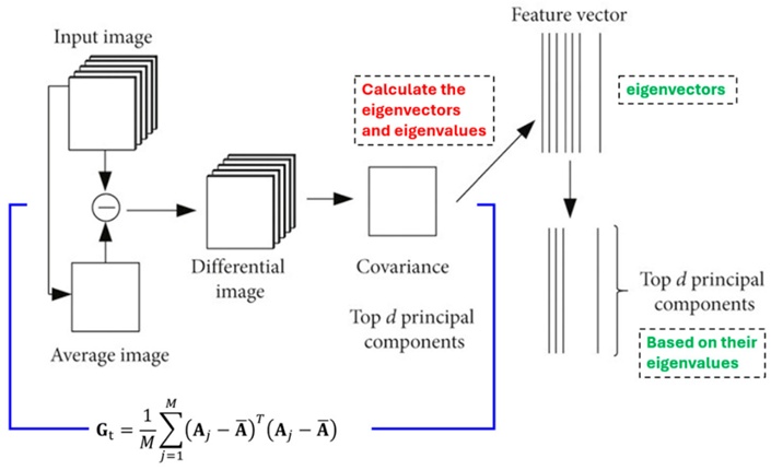
Figure 5. Graphical representation of the 2DPCA implementation (after Yin, Xiuye, and Chen) [47].
In this investigation, d was adjusted across a dynamic range to identify the optimal accuracy threshold based on models trained with varying quantities of principal components. However, the final ten eigenvectors were found to encode the majority of the structural image features, as shown in Figure 6.
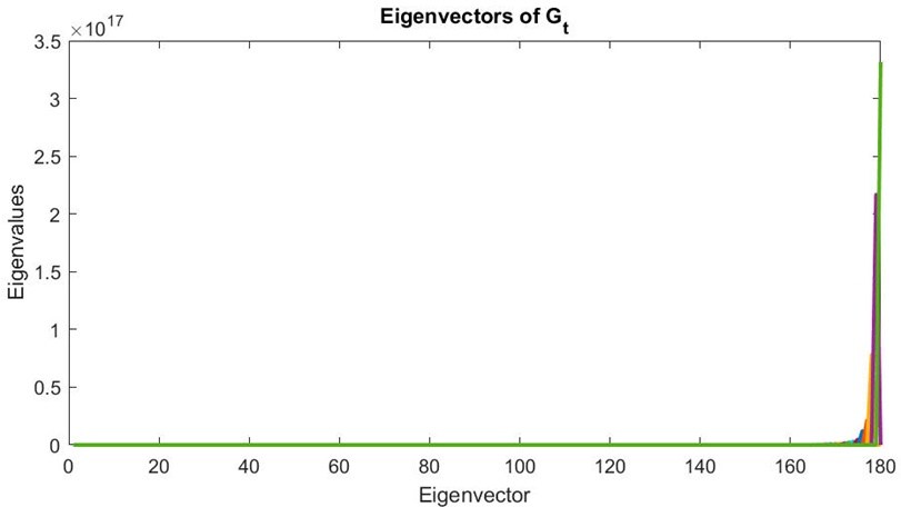
Figure 6. Eigenvectors of Gt with their corresponding eigenvalues. The last ten eigenvectors have the highest eigenvalues, with a noticeable difference compared to the other eigenvectors.
Feature extraction for any given image A is executed using the selected optimal projection vectors X1, . . . , Xd:
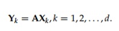 (11)
where Yk denotes kth vector among the projected feature vectors Y1, . . . , Yd, which are designated as the principal component vectors of Image A.
The extracted feature matrices belonging to the training dataset images are compiled as the reference database for subsequent classification tasks. A 2DPCA operation is likewise applied to every individual image within the testing dataset. Classification is thereafter executed using a nearest neighbor classifier by computing the distance metric between the feature matrix of the test image and each reference matrix stored in the database:
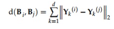 (12)
where , denote two arbitrary feature matrices corresponding to the test and training images, respectively, and − 2 represents the Euclidean distance between the two principal component vectors and .
Let the training set consist of the samples B1, B2, . . . , BM, where (M) denotes the total number of training samples. Each sample is associated with a particular class ωk. For a test sample (B), if = min and Bt ∈ ωk, then the classification outcome is B ∈ ωk. In the present study, a voting strategy based on the first three values was employed, as this approach contributed to improving the overall classification performance.
The resultant 2DPCA feature matrices for every image in the dataset were unrolled into a vectorized format to facilitate processing. These vectors, representing the characteristic features extracted via the 2DPCA method, were augmented with a final column to encode the classification category. This class variable was binarized as 0 for the "Empty" category and 1 for the "Event" category. These individual vectors were then concatenated into a master matrix where each row corresponds to a specific image sample and the terminal column provides the true class label. This consolidated matrix serves as the primary input for a machine learning framework that employs Recursive Feature Elimination (RFE) in tandem with a Random Forest classifier. This configuration is designed to quantify the specific influence of each principal component on the final predictive outcome.
Random Forest [48] is a prominent ensemble learning architecture frequently utilized in computational intelligence for its proficiency in addressing classification and regression challenges. The method operates by generating a large array of independent decision-tree classifiers. Each individual tree is developed using a random vector Θk, which is sampled independently while following a consistent distribution across the entire forest. The system synthesizes the individual tree outputs to improve overall predictive stability and precision. For classification problems, the Random Forest utilizes a majority-vote mechanism to determine the final class, whereas for regression, it averages the outputs from all trees. The core operational logic of the Random Forest relies on determining the margin function, assessing the robustness of constituent classifiers, and evaluating inter-tree correlation, as well as their collective impact on the model’s generalization error. These theoretical foundations allow Random Forests to maintain high performance, resist overfitting, and offer quantitative insights into variable importance, rendering it a highly resilient machine learning strategy.
The margin function, which serves as a metric for classification confidence, is expressed as:
 (13)
In this expression, h(X, Θ) signifies the output of an individual tree, denotes the probability measure associated with the random vectors \Theta, X represents the input data, and Y is the actual class label. An increased margin signifies a more confident classification result.
The collective strength of the forest is defined by the expected value of the margin function:
(14)
Here, s provides an evaluation of the mean performance of the individual trees within the ensemble.
The generalization error, indicating the likelihood of an incorrect classification, is constrained by the following upper bound:
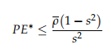 (15)
where represents the mean correlation between the various classifiers in the ensemble. This formula underscores the critical equilibrium between the accuracy of individual trees and their statistical independence, emphasizing that the success of a Random Forest depends on maximizing individual tree strength while minimizing inter-tree correlation.
RFE is a sophisticated feature selection methodology particularly effective for classification tasks involving limited sample sizes [49]. Initially utilized in the field of oncology for microarray-based classifications where the feature set significantly outnumbers the sample count (often fewer than 100), RFE has proven to be a robust tool for feature optimization. The technique prioritizes features by recursively fitting a model—in this study, a logistic regression—and pruning the least significant features in successive cycles until a predefined number of features is reached. This yields a definitive ranking of the original feature set based on their predictive value.
The research data was partitioned into training and validation subsets. The procedure commences with the ingestion of the training data and the application of 2DPCA to compress the high-dimensional imagery into a streamlined set of principal components, thereby retaining vital information in a condensed format. The efficacy of the 2DPCA is gauged by assessing a range of principal components associated with the highest eigenvalues to determine which specific subset maximizes detection accuracy. The training data corresponding to these high-performance components are then flattened and integrated into the RFE process alongside the Random Forest model. Here, the Random Forest serves as the base estimator for the RFE cycle. RFE systematically removes the least impactful features according to the importance metrics generated by the Random Forest, iteratively refining the feature set to the optimal count. In each cycle, feature importance is distilled across the components to calculate their total contribution to the system’s logic. The final output consists of prioritized importance rankings and graphical representations showing the percentage impact of various features on classification. These procedural steps ensure the model achieves superior accuracy while providing transparent insights into the components influencing its predictions, consistent with XAI objectives. Finally, the three most significant components are isolated to build the definitive model, reaching peak accuracy with the most efficient model size. The procedural flowchart is presented in Figure 7.
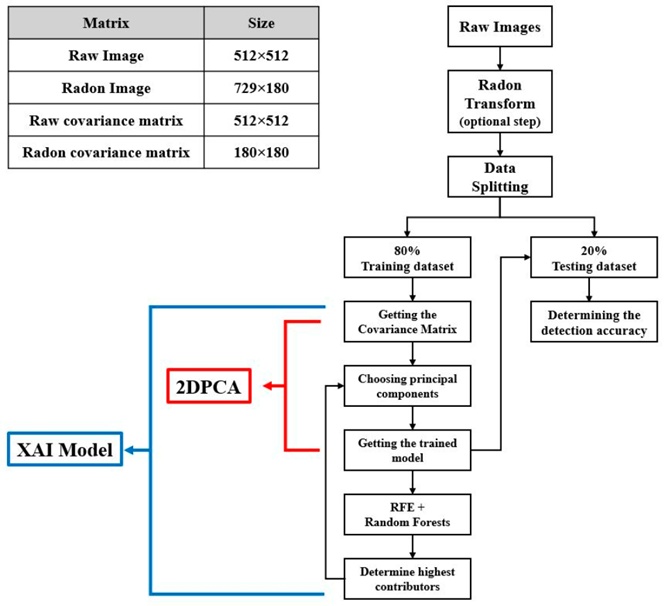
Figure 7. Flowchart of the XAI model with a table of matrix sizes in the upper left corner.
The metrics employed to evaluate the predictive performance of the models are defined below:
Accuracy quantifies the global effectiveness of the system by calculating the ratio of correct classifications to the total number of evaluated samples:
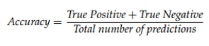 (16)
In this context, True Positive refers to instances where the model correctly identified an EPB that was physically present. True Negative refers to cases where the model correctly identified the absence of an EPB in a clear image.
Precision measures the reliability of positive results by determining the ratio of correctly identified EPBs (True Positives) against the total number of positive flags issued by the model:
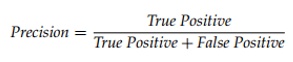 (17)
where False Positive denotes cases where the model incorrectly flagged a bubble in an image that did not contain one.
Recall determines the model’s sensitivity to positive cases by calculating the ratio of True Positives relative to the sum of True Positives and False Negatives:
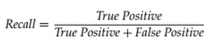 (18)
where False Negative signifies a missed detection—an instance where the model failed to recognize an existing EPB.
The F1-score provides a comprehensive performance metric by harmonizing precision and recall into a single value:
 (19)
The standard 2DPCA model, configured without the Radon transform, underwent multiple training cycles using the training data. Each cycle utilized a differing quantity of the primary principal components, corresponding to various thresholds of the dataset’s total eigenvalues. This cut-off was maintained at a minimum of 95%. The model was subsequently validated using a testing dataset that was selected at random and remained static for all comparative tests. The validation results demonstrated non-linear fluctuations in accuracy; contrary to theoretical expectations, an increase in the captured percentage of eigenvalues did not always yield a proportional improvement in feature performance (per Yang and Yang) [46]. This variability may be attributed to the inherent characteristics of the dataset, which comprises airglow imagery captured under diverse atmospheric and geomagnetic conditions. External factors such as cloud density, background noise, and varying observational constraints can introduce inconsistencies that influence model stability across different test iterations.
Table 1 outlines the number of selected eigenvectors with the highest eigenvalues, their percentage relative to the total eigenvalue sum, the resulting accuracy, and the training time required for the 1967-image training set.
Table 1. Detection accuracy based on 2DPCA without using Radon transform.
Number of Principal Components | Elapsed Time (s) | Accuracy (%) | Eigenvalues Cut (%) |
20 | 301.692 | 96.95 | 97.57 |
30 | 301.748 | 97.96 | 98.43 |
40 | 301.705 | 96.54 | 98.86 |
50 | 301.896 | 96.54 | 99.13 |
60 | 301.766 | 97.15 | 99.31 |
70 | 301.918 | 97.35 | 99.44 |
80 | 301.916 | 96.95 | 99.54 |
90 | 301.879 | 97.15 | 99.62 |
The 2DPCA architecture was then retrained following the same parameters but after the application of the Radon transform. Pre-processing images via this transform adjusted the resolution from 512 \times 512 pixels to 729 \times 180 pixels. This resulted in a more compact covariance matrix, utilizing only 180 eigenvectors compared to the original 512. This shift allowed a smaller number of eigenvectors to represent the same eigenvalue thresholds as the previous trial, markedly decreasing both the training time and the final model footprint. However, the use of the Radon transform on raw imagery led to a slight decline in overall detection accuracy. Table 2 presents the feature contribution percentages, training durations, and accuracy levels for various eigenvector selections.
Figure 8 provides a visual comparison of the data presented in Tables 1 and 2. The horizontal axis indicates the eigenvalue cut-off percentages for the principal components used in training, while the vertical axis shows the corresponding accuracy. The specific number of principal components employed for each 2DPCA iteration is noted above each data point. The visualization confirms that models trained on raw data consistently outperform those using Radon-transformed data. Specifically, for raw data, the model using the thirty highest principal components reached a peak accuracy of 97.96%. For the Radon-transformed data, the model using the top ten principal components reached a peak accuracy of 96.1%. These high-performance models are indicated by green circles.
Table 2. Detection accuracy based on 2DPCA using Radon transform.
Number of Principal Components | Elapsed Time (s) | Accuracy (%) | Eigenvalues Cut (%) |
3 | 130.660 | 94.30 | 99.48 |
4 | 130.678 | 94.70 | 99.64 |
5 | 130.673 | 94.50 | 99.73 |
10 | 130.683 | 96.13 | 99.90 |
15 | 130.793 | 93.89 | 99.95 |
20 | 130.751 | 93.89 | 99.97 |
25 | 130.873 | 93.89 | 99.98 |
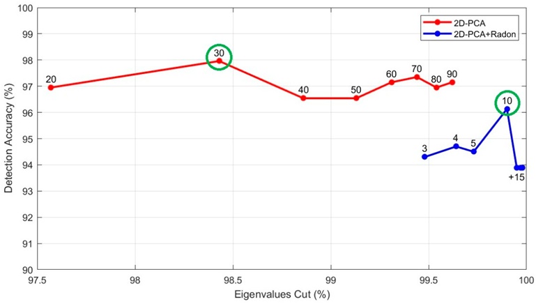
Figure 8. Detection accuracy versus eigenvalue cut-off using different numbers of principal components to train 2DPCA models with raw images (red) and Radon-transformed images (blue). The highest detection accuracies are highlighted with a green circle.
RFE was subsequently combined with the Random Forest classifier and applied directly to the most accurate model variants from each case. This step was conducted to isolate and quantify the specific prognostic weight of individual principal components during the image classification task. The specific eigenvalues for each principal component are outlined in Figure 9a. In parallel, Figure 9b maps the precise percentage contribution of each principal component toward identifying the correct class of the validation frames, as determined by the RFE and Random Forest pipeline. Cross-examination of these two panels reveals that the principal components carrying the largest eigenvalues do not automatically possess the greatest predictive relevance during the classification stage. For example, the 30th principal component, despite exhibiting the lowest eigenvalue, emerged as the most critical variable within the classification architecture. In an identical manner, Figures 9c and 9d present the principal component eigenvalues for the configuration built on Radon-transformed data alongside their respective percent contributions to the classification task. Even though the tenth and ninth eigenvectors possess the lowest eigenvalues, their corresponding principal components ranked as the first and third most influential parameters within the decision-making pipeline, respectively.
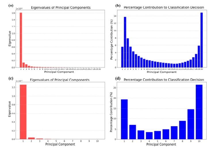
Figure 9. (a) Eigenvalues of each principal component in the XAI model. (b) Actual contribution of each principal component to the classification process. (c,d) Represent the same as (a,b) but for the XAI (Radon) model.
The developed XAI framework categorizes the principal components according to their verified operational contribution. It then leverages 2DPCA to sequentially introduce these principal components into the training workflow based on their updated significance hierarchy before validating the performance on the testing subset. Following this, the system documents the quantity of active principal components alongside the resulting classification accuracy. Ultimately, it isolates the specific model configuration that yields the maximum detection accuracy while preserving the smallest possible data footprint. This sequential optimization routine is detailed in Figure 10. The updated optimal configurations were established using the top thirteen principal component drivers for the raw data pipeline and the top three drivers for the Radon-transformed pipeline. These optimized configurations demonstrated a detection accuracy improvement of 0.21% for the raw image architecture, ascending to 98.17%, and an improvement of 1.22% for the Radon-transformed framework, climbing to 97.35%. Furthermore, these configurations exhibited a vastly compressed structural footprint relative to the baseline models, achieving structural size reductions of 56.6% and 70% for the raw and Radon-transformed pipelines, respectively.
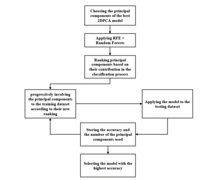
Figure 10. Flowchart of the combination process of 2DPCA and Random Forest in conjunction with RFE.
To rigorously evaluate its capability, the proposed framework was benchmarked against established deep learning baseline models, specifically ResNet18, Inception-V3, VGG16, and VGG19 [50, 51]. These CNN architectures were trained using the previously described data partition split from scratch without using transfer learning, thereby preserving their native architectural frameworks. To guarantee an equitable comparison, all candidate networks were trained within an identical computing environment. Furthermore, matching hyperparameters were applied across all runs, utilizing a fixed batch size of 16. The training threshold was capped at 10 epochs to limit total computational runtime while preserving the ability to isolate and extract the specific epoch that yielded peak validation accuracy alongside the lowest training loss. The primary training database partition was split into localized training and validation subsets, allocating 80% for training parameters and 20% for validation tracking. All data arrangements remained uniform across every tested model. The diagnostic throughput of each network was measured via the metrics. The derived evaluation parameters for all tested frameworks are summarized in Table 3.
Table 3. Model evaluation results for the EPB detection of different deep learning models, the proposed 2DPCA, and XAI models.
Model | Elapsed Time (min) | F1-Score (%) | Sensitivity (%) | Precision (%) | Accuracy (%) |
ResNet18 | 38.72 | 92.05 | 91.36 | 92.76 | 91.45 |
Inception-V3 | 114.30 | 90.04 | 89.32 | 90.78 | 89.41 |
VGG16 | 215.70 | 86.74 | 85.19 | 88.35 | 85.34 |
VGG19 | 255.96 | 89.83 | 89.33 | 90.32 | 89.41 |
2DPCA | 5.03 | 97.99 | 97.95 | 98.03 | 97.96 |
2DPCA (Radon) | 2.18 | 96.27 | 96.17 | 96.37 | 96.13 |
XAI | 8.71 | 98.17 | 98.16 | 98.18 | 98.17 |
XAI (Radon) | 3.03 | 97.40 | 97.38 | 97.43 | 97.35 |
The metrics detailed in Table 3 are graphically visualized in Figure 11. Figure 11a emphasizes the operational variations among the newly developed models, illustrating the direct relationship between classification accuracy and cumulative training time. Figure 11b displays the identical relationship while incorporating the deep learning CNN architectures for broader context. The visual comparison reveals that peak detection accuracy was accomplished by the raw-data-driven XAI model, which achieved a 98.17% success rate and outperformed all other proposed variations as well as the deep learning networks, whereas the lowest overall accuracy was generated by VGG16.
Nonetheless, the XAI model leveraging Radon-transformed imagery showed the most efficient performance profile when balancing classification accuracy against training runtime. While it secured the second-highest accuracy score—differing from the leading model by a mere 0.82%—it drastically minimized the temporal requirement, demanding only 35% of the training time consumed by the top-performing raw image model. Furthermore, the proposed 2DPCA feature extraction technique required a fraction of the training time demanded by the deep learning networks operating under identical environmental conditions. Although integrating the XAI layer brought a minor increase in training latency compared to standalone 2DPCA, it yielded notable improvements in classification accuracy alongside a marked reduction in the final model file size. Deploying the proposed XAI architecture with minimized operational latency facilitates the construction of compact, rapidly trained diagnostic tools that draw minimal computational energy while maintaining high accuracy thresholds. Such streamlined models are highly appropriate for integration within real-time tracking software and deployment on low-cost hardware platforms.
However, the architecture can exhibit sensitivity to partially cloudy sky conditions, particularly when a single frame captures both plasma bubbles and localized cloud formations simultaneously. This mixture can trigger false classifications or a failure to distinguish legitimate plasma bubbles due to spatial obstructions during real-time tracking. Despite this environmental constraint, equatorial plasma bubbles tend to persist within the imager's field of view significantly longer than passing cloud structures. This behavioral difference permits a more resilient diagnostic approach founded on consensus decisions across sequential ASI frames, thereby mitigating false positives and raising total classification accuracy.
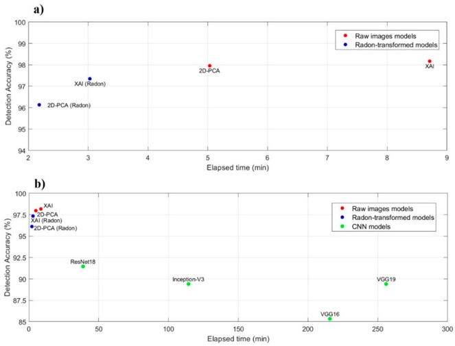
Figure 11. (a) Differences among the proposed models, showing detection accuracy plotted against elapsed training time. (b) The same comparison, including deep learning CNN models.
In this investigation, a computationally efficient XAI model was engineered for the automated detection of equatorial plasma bubbles within ASI datasets. This framework was built by pairing 2DPCA with RFE alongside a Random Forest machine learning classifier. A database comprising 2458 ASI frames was gathered and manually sorted into two core classes: the “Empty” class for frames devoid of plasma bubbles, and the “Event” class for frames where a plasma bubble manifests. This image collection was partitioned into a 80% training subset and a 20% testing subset, which were kept uniform across all comparative runs. The baseline trial was conducted by applying 2DPCA directly to the raw image data, which achieved a detection accuracy of 97.96%. Introducing the Radon transform in subsequent testing cycles succeeded in reducing the computational training time and compressing the structural model size by nearly 65%, though it lowered the baseline detection accuracy to 96.1%.
The XAI model was subsequently leveraged by extracting the eigenvectors from the most accurate model configurations to determine the actual diagnostic contribution of each principal component during classification. These components were prioritized by contribution percentage via the RFE and Random Forest pipeline. Guided by this updated ranking, the principal components were step-by-step integrated into the 2DPCA training framework to construct an optimized model that maximizes detection accuracy while minimizing its data footprint. Although the inclusion of the XAI layer marginally increased processing time relative to standalone 2DPCA, it enhanced the accuracy of the raw-image model by 0.21% (reaching 98.17%) and raised the accuracy of the Radon-transformed model by 1.22% (reaching 97.35%). It simultaneously minimized the storage requirements of the trained detection models compared to standard 2DPCA, yielding size reductions of 56.6% for the raw image framework and 70% for the Radon-transformed framework.
Furthermore, cross-comparisons with deep learning CNN networks demonstrated the superiority of the proposed models regarding both classification accuracy on raw ASI imagery and total training speed. The highest detection accuracy among the deep learning baseline networks was achieved by ResNet18 at 91.45%, placing it 4.68% to 6.72% behind the proposed frameworks. Additionally, ResNet18 proved to be the fastest deep learning model, requiring 38.72 minutes to train across 10 epochs, whereas the proposed frameworks required only 2.18 to 8.71 minutes to complete training within the same computing environment. The proposed models are highly suited for incorporation into real-time tracking pipelines and installation on low-cost hardware systems. While the system may display sensitivity to partially cloudy conditions that can induce misclassifications, EPBs remain within the ASI field of view for extended intervals. This temporal persistence enables accuracy enhancement through collaborative decision-making across multiple sequential ASI frames, thereby suppressing false alarms and optimizing overall performance.
The following abbreviations are used in this manuscript:
2DPCA | Two-Dimensional Principal Component Analysis |
ASI | All-Sky Imager |
BJL | Bom Jesus da Lapa Observatory |
CA | São João do Cariri Observ |
CCD | Charged Coupled Device |
CDF | Cumulative Distribution Function |
CNN | Convolutional Neural Network |
EPBs | Equatorial Plasma Bubbles |
RF | Random Forest |
RFE | Recursive Feature Elimination |
This work was supported by the SCOSTEP Visiting Scholar (SVS) program of the Scientific Committee on Solar-Terrestrial Physics (SCOSTEP), for which the first author stayed for three months at the Institute for Space-Earth Environmental Research, Nagoya University. Further- more, the authors thank the Embrace/INPE Space Weather Program for their dedicated efforts to provide substantial data to study the ionosphere around the magnetic equator.
None
None
None
Open Access The author(s) retain copyright. This article is licensed under the Creative Commons Attribution-NonCommercial-ShareAlike 4.0 International License. It may be shared and adapted for non-commercial purposes with appropriate attribution, an indication of changes, and distribution of adaptations under the same license. Third-party material may be subject to separate terms identified in its credit line. View the license at https://creativecommons.org/licenses/by-nc-sa/4.0/.
 Transparent Intelligence Publishing