This research investigates and refines the MINDWALC node classification algorithm, specifically targeting its capacity to extract human-interpretable decision trees from knowledge graph (KG) architectures. We propose techniques to tailor MINDWALC for environments where the knowledge graph is bifurcated into internal background knowledge (domain-specific data) and instance knowledge (specific case data). While the core logic of MINDWALC—utilizing discriminative graph walks as features—is preserved, we introduce two primary enhancements. First, we implement relation-tail merging to empower the algorithm to process relation-modified nodes. Second, we propose flexible walking depths that, when combined with the original MINDWALC strategy, improve the detection of commonalities between node instances. Our findings suggest that these flexible walks can markedly increase classification accuracy in hierarchical or incomplete tree-like graphs, though performance varies on more heterogeneous KG structures. Ultimately, this work demonstrates that our refinements significantly boost MINDWALC’s utility in tree-structured environments, allowing the system to use background knowledge to bridge gaps in instance data in a transparent way. Initial evaluations on medical toy datasets suggest these optimizations could refine clinical decision-making, particularly in sectors requiring explainable artificial intelligence.
In the contemporary medical landscape, maintaining clinical competency is increasingly difficult due to the exponential growth of data across all specialties. Within surgical pathology—the primary field of the authors—new disease entities and sub-classifications are frequently identified. Furthermore, diagnostic frameworks and nomenclatures undergo constant revision, as seen in the periodic updates to the World Health Organization (WHO) blue book series. Consequently, medical professionals and diagnosticians must engage in continuous professional development to provide high-quality care. Given that pathologists are essential to oncology—establishing the definitive diagnoses and cancer staging that dictate patient management—staying current is a vital prerequisite for favorable clinical outcomes. This rapid expansion of knowledge presents a formidable challenge for the individual practitioner.
Pathologists are expected to synthesize information from standard reference texts with the latest peer-reviewed findings (e.g., via Pubmed) to arrive at standardized, justifiable conclusions. Such a process requires a systematic set of rules to evaluate competing clinical features. Standard medical literature typically presents this information in either narrative prose or as tabular summaries of evidence supporting or contradicting a specific diagnosis. For instance, the WHO volume "Classification of Tumors of Hematopoietic and Lymphoid Tissues" requires significant revisions for every edition to incorporate burgeoning scientific data [1]. This constant integration leads to larger volumes and a higher number of potential differential diagnoses. While these texts highlight essential diagnostic markers, practitioners must often develop bespoke diagnostic algorithms to solve complex cases, such as distinguishing follicular lymphoma with aberrant CD5 expression from mantle cell lymphoma [1]. Resolving these specific challenges often requires targeted literature reviews via databases like Pubmed.
In this context, diagnostic tools such as mind maps or decision trees—mirroring the checklists used in the aviation industry—could be highly effective. While various expert-derived algorithms exist for educational purposes, such as "Mind Maps for Medical Students Clinical Specialties" [2], they are rarely developed for board-certified specialists managing intricate cases. The lack of standardized checklists for rare or complex differential diagnoses is likely due to structural hurdles: experts capable of designing these algorithms are few and time-constrained, and the labor required to keep such tools updated is immense, rivaling the complexity of the WHO blue book series itself.
This necessitates an automated approach. In this article, we demonstrate how the MINDWALC algorithm [3], combined with a curated, domain-specific Knowledge Graph (KG), can be used to generate interpretable decision trees. Since high-quality, comprehensive KGs are difficult to obtain, we utilize "toy" datasets that contain the necessary information for classification while remaining accessible to a general audience.
Initially, we utilize a dataset from "geek culture"—the Pokemon franchise—as it offers high-quality, community-vetted data that is intuitively understandable. In this model, creatures possess elemental types (e.g., fire, water) that dictate their interactions through logical rules (e.g., water's advantage over fire). Insights from these experiments allowed us to identify MINDWALC’s limitations, which we addressed through relation-tail merging and flexible walking depths. We then validated these optimizations on a synthetic medical dataset designed for diagnosing prostate adenocarcinoma. Finally, we benchmarked our enhanced MINDWALC against contemporary deep learning node classification models using real-world graph data.
The fundamental concept underpinning knowledge graphs—which involves archiving interconnected concepts rather than basic text strings—is not new. This methodology originated in the late 1970s and was subsequently revitalized by technology corporations, spearheaded by Google, during the 2010s [4, 5]. Despite its long-standing history, knowledge graphs have not achieved uniform standardization, resulting in diverse operational definitions and conceptual interpretations across the field [4, 6].
A primary benefit of rigorously maintained knowledge graphs is their capacity to represent facts and data in an explicit, unambiguous manner that is legible to both human users and computational systems. While contemporary transformer-based language models demonstrate remarkable proficiency in extracting and parsing information from unstructured textual documents, graph-structured knowledge inherently minimizes the potential for linguistic misinterpretation. Consequently, there is a growing trend to integrate KGs as a supplementary modality alongside existing Artificial Intelligence (AI) frameworks to optimize model performance. For example, Agrawal et al. [7] detailed several implementations where knowledge graphs serve to mitigate hallucination phenomena in conversational agents. Similarly, within the K-PathVQA framework [8], incorporating a KG enhanced the diagnostic accuracy of a pathological Vision Question Answering (VQA) system. However, that study also demonstrated that the fidelity of the provided graph is critical, noting that an out-of-domain KG can degrade performance compared to configurations utilizing no supportive graph at all.
Numerous state-of-the-art deep learning models exist for interpreting relational graph data, such as Relational Graph Convolutional Networks (R-GCN) [9] and RDF2Vec [10]. Nonetheless, these deep learning methodologies function essentially as black boxes, preventing users from directly auditing the underlying logic that leads to a specific prediction. Generating explanations from these models typically demands post-hoc analytical procedures to isolate the specific subgraphs or nodes responsible for a given output, which are then rendered into a human-readable visual format. Conversely, the present study utilizes the MINDWALC algorithm [3], which operates directly on knowledge graphs without requiring embedding steps. This characteristic ensures that the entire diagnostic pathway and the generated decision tree remain fully transparent and interpretable.
MINDWALC operates as an interpretable node classification architecture centered on mining discriminative walks across a targeted KG. Each walk originates at the target classification nodes (instances) and traverses outwards into the broader graph structure. Every individual path functions as a human-readable feature suitable for training a decision tree model. Because each decision node within the finalized tree corresponds directly to a distinct graph walk, the overall model maintains intrinsic interpretability. Although this approach bypasses computationally heavy deep learning mechanisms, Vandewiele et al. demonstrated that it achieves competitive classification metrics while preserving absolute transparency [3].
Following the taxonomies outlined in [11], the MINDWALC framework is classified under Interpretable Machine Learning (IML). This classification applies because the model does not merely generate an ex-post explanation of its outputs; it functions inherently as an interpretable white-box architecture by design.
Rule mining techniques offer another prominent example of IML applied to knowledge graphs, sharing similarities with the MINDWALC framework. The Path Ranking Algorithm (PRA) [12] and its contemporary iterations or enhancements (such as RDF2rules [13], AIME+ [14], Ontology Pathfinding (OP) [15], and SAFRAN [16]) were engineered primarily for knowledge graph completion and link prediction tasks. These methods map paths across a knowledge graph to deduce which relations typically manifest when specific path structures are present. For instance, if a path follows the sequence \text{(person)} \xrightarrow{\text{works\_for}} \text{(company)} \xrightarrow{\text{resident\_in}} \text{(city)}, the system infers the existence of the relation \text{(person)} \xrightarrow{\text{works\_in}} \text{(city)}. However, PRA can also be adapted for node feature extraction by utilizing path-type frequency vectors as descriptive node attributes [11]. MINDWALC employs a conceptually similar routine but differs by implementing alternative graph-traversal strategies, which directly influence the dimensionality of the resulting feature vectors. Furthermore, while PRA relies on logistic regression to learn rule clauses, MINDWALC leverages decision tree classifiers to isolate the most informative and discriminative graph pathways.
Additionally, the semantic decision tree framework presented by Jeon et al. [17] represents a compelling alternative for deriving interpretable decision boundaries from graph structures. However, in contrast to MINDWALC, that method is tailored specifically for binary node classification tasks and constructs decision trees via rule expressions—defined as sequential chains of conditions that must all evaluate to true to return a positive prediction. To scale semantic decision trees for k-class classification problems, one would need to train and integrate k separate semantic decision trees, as demonstrated in [18].
Another critical aspect of MINDWALC is its inability to run directly on raw relational graphs; instead, it operates indirectly by converting the target relational graph into a non-relational counterpart. This structural transformation introduces certain limitations in specific contexts, which are analyzed and partially mitigated in Section 2.5 of this study.
It is vital to emphasize that our research focuses on optimizing MINDWALC for a highly specific operational scenario. This architectural configuration is illustrated in Figure 1.
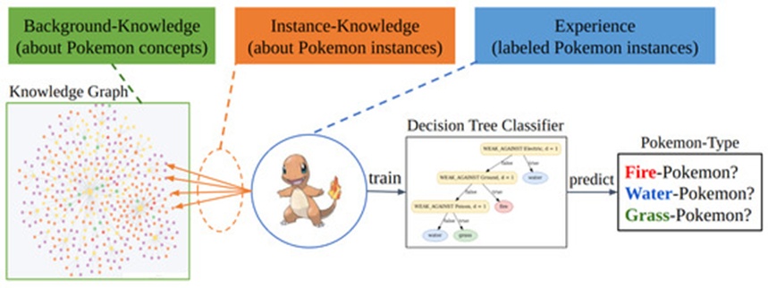
Figure 1. The three main components of the investigated system. This work aims to use and optimize the MINDWALC node classifier for the following specific use-case system. The most important idea is to divide the given graph on which MINDWALC operates into three components: first, the inner background knowledge (green), which describes how domain-specific concepts are related to each other; second, the experience (blue), which is represented by labeled instance nodes (nodes to classify). third, the instance knowledge (orange), which is represented by specific relations which connect each node instance with multiple concept nodes from the background knowledge graph. The idea is to classify the node instances of such a system using a MINDWALC decision tree classification in order to generate human-interpretable decision trees during training.
The core principle of our operational setup is that the processed graph is consistently segregated into three distinct components. Each component serves a distinct purpose and represents a foundational phase of the decision-making pipeline:
Background Knowledge: The background knowledge constitutes the internal core of the KG and maps the relationships between various domain-specific concepts. In the context of the Pokemon domain, it models how different structural concepts (such as attributes, special abilities, move sets, and team compositions) interface with one another. Within a medical context, this background layer might manifest as a clinical ontology delineating the connections between various medical terms and pathologies. Because the background knowledge graph establishes the baseline rules and principles of the target domain, it is essential that this data remains free of factual errors to prevent the model from deriving invalid conclusions during classification.
Experience: The corpus of labeled instance nodes serves as the explicit experience of the classification framework. Consequently, within our experimental setup, expanding the volume of labeled Pokemon nodes (instances) increases the experience available to the model, which typically yields a measurable improvement in overall classification accuracy.
Instance Knowledge: Instance knowledge characterizes the specific attributes of individual entities—for example, mapping which explicit Pokemon instances possess specific abilities, belong to particular groups, or display distinct vulnerabilities and resistances. This data is established by the primary relations that anchor each individual Pokemon node to the core background knowledge graph. In real-world applications, instance knowledge may suffer from inconsistencies or incomplete data, given that extracting information for every unique instance is subject to collection errors. In a clinical environment, individual patient cases serve as instances defined by unique client records (instance knowledge). This specific case information may occasionally lack the resolution or detail required to generate a definitive diagnosis on its own.
When evaluating human decision-making processes, it is entirely feasible to execute intuitive judgements relying solely on direct experience and localized instance data without consulting broader theoretical frameworks. However, diagnostic accuracy and reliability generally improve when leveraging established background knowledge acquired through formal education or extracted from authoritative reference literature.
Having defined the architecture and functional roles of these three graph components, we can outline how they are synthesized with machine learning to categorize node instances and construct decision trees. As illustrated from left to right in Figure 1, the pipeline requires an established background knowledge graph; subsequently, labeled entities and their corresponding instance knowledge are compiled to link these entries to the background structure using explicitly defined relations. We then train a decision tree-based node classifier that leverages both the immediate instance properties and the deeper, underlying background knowledge to assign target labels to the instances. Following model training, we analyze the resulting decision trees to evaluate their level of human comprehensibility.
The MINDWALC node classification paradigm is uniquely suited for this specific application because it can systematically traverse the initial instance knowledge layer and penetrate deeper into the underlying background knowledge in a completely transparent manner. A particularly compelling area of study is determining the exact depth the classifier reaches within the KG to make a prediction. Pathways exceeding a single step extend directly into the domain of background knowledge. Decisions derived from these deeper trajectories are no longer purely instinctive reactions based on immediate experience; instead, they reflect logical deduction and chained reasoning. Increased walk depth corresponds to a longer and more intricate sequence of synthesized conclusions. The primary catalyst for adopting this framework is its strict demarcation between background knowledge, instance knowledge, and experience, alongside the structural transparency of the resulting decision pathways.
To assess the efficacy of different methodologies across various graph architectures and node classification tasks, seven specific multi-relational graphs were evaluated: three Pokemon-based knowledge graphs, one synthetically generated medical graph, and three real-world benchmark datasets. An initial summary of these graph characteristics is detailed in Table 1.
Table 1. Properties of examined knowledge graphs. Node and relation count of all seven multi-relational graphs which have been examined in this work. Train-test entities indicates how many labeled nodes are available in the graph, which are used to train and test different MINDWALC node classifiers.
Train-Test Entities | Relation Count | Node Count | |
GottaGraphEmAll | 139 | 47,988 | 4160 |
TreeOfLife | 44 | 850 | 851 |
CombinedPokemon | 104 | 48,980 | 4496 |
ProstateToyGraph | 444 | 7909 | 2702 |
AIFB | 178 | 29,226 | 8285 |
BGS | 146 | 916,421 | 333,863 |
MUTAG | 340 | 74,567 | 23,644 |
The GottaGraphEmAll network functions as our model for a property-based graph layout. Originally distributed as a Neo4J graph database by [19], its architectural blueprint (Figure 2) illustrates the systemic features mapping individual Pokemon (including movesets, intrinsic abilities, vulnerabilities, and elemental strengths). We classify this schema as a property-based knowledge graph because its primary objective is defining specific attributes and mapping the network configurations between these attributes and the entities.
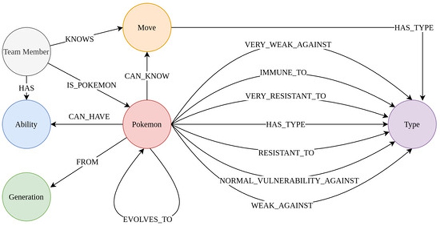
Figure 2. The schema of the knowledge graph GottaGraphEmAll. The schema of the Pokemon graph GottaGraphEmAll. As we can see, this knowledge graph describes how different Pokemon are related to different Pokemon types, team members, abilities, generations, and moves.
Certain knowledge graphs utilize a hierarchical taxonomy where individual nodes branch into multiple sub-nodes, producing a tree-like topology. Multiple medical classification systems, including Kidney Biopsy Codes (KBC) [20], the Unified Medical Language System (UMLS) [21], and Snomed CT [22], leverage hierarchically structured terms that form an incomplete tree. As a domain-specific surrogate for a hierarchical model, the phylogenetic and evolutionary tree of life engineered by Shelomi et al. [23] was adapted into a Neo4J graph format. As illustrated in Figure 3, this tree of life structure binds individual Pokemon nodes (represented as leaf nodes) to broader ancestral classification groups.
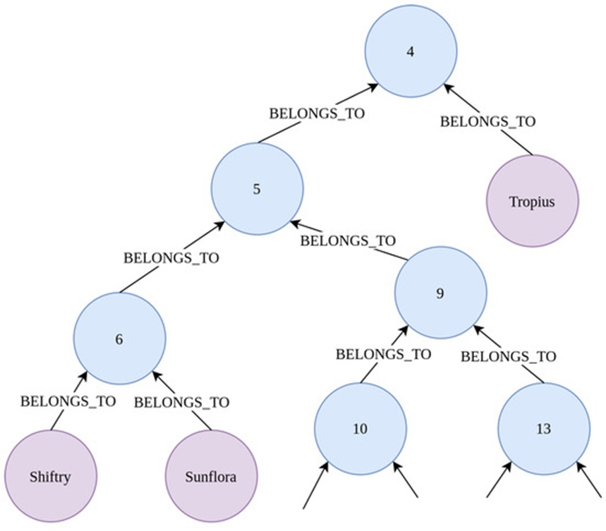
Figure 3. Small part of the tree of life Pokemon graph. As we can see, the tree of life Pokemon graph has a tree-like structure. Each Pokemon node (purple nodes) is a leaf of the tree and belongs to multiple PokeCategory nodes (blue nodes, named with random category numbers). This tree of life graph was generated in [23] and the Pokemon grouping is based on anatomical properties and other Pokemon attributes.
To evaluate the capabilities of our optimized MINDWALC framework on hybrid topologies, the property-based graph and the hierarchical graph were integrated into a single unified dataset. This integration reflects real-world deployment scenarios where maximizing consolidated data within a single knowledge repository is advantageous. The sole overlapping elements between the two networks were the core Pokemon nodes. During the fusion process, duplicates were resolved to guarantee each entity was uniquely represented, and any instance lacking a presence in both source networks was removed.
To assess model viability within a specialized medical framework, we constructed a synthetic knowledge base focused on prostate adenocarcinoma. Relevant clinical concepts were initially derived from the Snomed CT ontology. We then supplemented this framework by manually incorporating missing clinical nodes and medical relationships, guided by professional pathological expertise and academic reference manuals. The finalized knowledge graph is accessible via our public GitHub repository.
Subsequently, we generated a series of synthetic pathological patient cases. Each distinct case is represented as an independent node instance assigned to one of four diagnostic categories:
adenocarcinoma (GP3-5)
GP3 mimicker
GP4 mimicker
GP5 mimicker
Our pathology consultants curated a diagnostic feature inventory for each class, detailing the clinical criteria that typically manifest within that specific diagnosis. Using a custom script, we produced 111 case node instances per diagnostic category. Each generated node was randomly linked to between 10% and 100% of the target concepts within its assigned class using edges designated as DETECTED.
To benchmark our optimization strategies against authentic data, we utilized three standard graph repositories: AIFB, BGS, and MUTAG. These exact networks were evaluated in the foundational MINDWALC study by Vandewiele et al. [3] and are accessible via the repository curated by Ristoski et al. [24]. Structural metrics for these networks are indexed in Table 1.
The AIFB network maps the institutional connections between research personnel, distinct departments, ongoing projects, and corporate workflows. The classification objective is to predict the specific research group assignment for individual scientists. The BGS repository details geological attributes across 146 distinct rock formations, where the machine learning goal is to categorize samples as either fluvial or glacial deposits. The MUTAG network contains biochemical structures representing 340 complex molecular compounds, with the classification task focused on predicting whether a given molecule exhibits potential mutagenic characteristics.
This section outlines the basic methodology of the MINDWALC framework. This technical summary addresses its foundational mechanisms at a high level; exhaustive implementation details are documented in the original publication [3]. The diagram in Figure 4 simplifies the complete operational workflow of the MINDWALC decision tree model. The framework is divided into three primary functional phases (I, II, and III):
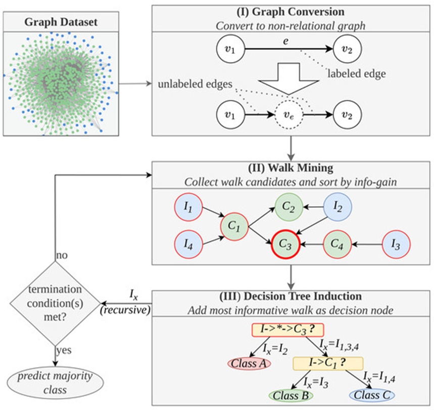
Figure 4. Methodical overview of MINDWALC decision tree classification. (I) The MINDWALC data processing pipeline begins by converting a relational knowledge graph into a non-relational graph by transforming each relation into a node. (II) The second step is the primary concept of MINDWALC, which involves mining walks through the graph. Each walk starts from the node instances (𝐼1−4, blue nodes) and proceeds through the graph until a certain target concept node (𝐶1−4, green nodes) is reached. The information gain of each walk is calculated (see [3] for details). The most informative walk is used to generate the next decision tree node. (III) A binary decision tree is built recursively from top to bottom. Each decision node (yellow) splits the given instances into two groups based on whether they can complete a particular walk (right child) or not (left child). The notation 𝐼→∗→…→𝐶𝑥 in the decision nodes describes the corresponding walks that start at the instances I and end at a target node Cx. All nodes in between can be any node and are marked with ∗, as defined in Formula (1).
As detailed in [3], MINDWALC requires a directed, multi-relational knowledge graph as its initial input, defined as:
𝐺=(𝑉,𝐸,ℓ)
Here, vertices 𝑣∈𝑉 and directed edges 𝑒∈𝐸 within the graph G are annotated using a labeling function, ℓ. To minimize architectural complexity, the initial phase of the MINDWALC pipeline converts this relational graph into a non-relational format. This is achieved by mapping each discrete relation e into a corresponding node v_e, as illustrated in Figure 4(I). This architectural conversion introduces specific structural constraints.
The secondary module, designated as phase (II) in Figure 4, constitutes the core mechanism of the MINDWALC framework: extracting and compiling localized paths, termed walks (w). Each distinct path originates at a targeted instance node (I) and evaluates directional paths across the converted non-relational KG. As defined in [3], such a path is mathematically formulated as:
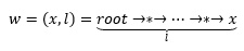 (1)
where 𝑟𝑜𝑜𝑡 designates the starting instance node slated for classification, l denotes the explicit walk depth, and x represents the terminal target concept node within the KG. Thus, any given walk can be uniquely represented as a tuple:
w=(x,l)
The walk mining procedure operates through a systematic routine. First, the algorithm gathers all viable candidate paths that can be traversed by at least one active instance node. For every candidate path, an information gain metric is computed by assessing which instances can successfully execute the walk versus those that cannot (refer to equation 4 in [3]). As shown in Figure 4(II), instances (𝐼1,2,3,4) capable of successfully traversing the path 𝑤=(𝐶3,2)=𝑟𝑜𝑜𝑡→∗→𝐶3 are highlighted. If the subpopulation of instances that successfully complete a specific walk maps directly to a uniform target class, that walk receives a proportionally high information gain value.
To construct a binary decision framework, each decision node within the tree is recursively generated using a top-down approach. Each node evaluates the most discriminative walk candidate and checks whether an instance can successfully execute that specific path. This mechanism splits the instances into two paths: those that can complete the walk (the right branch) and those that cannot (the left branch). This partitioning continues until one of three termination conditions defined in [3] is reached: all remaining instances share an identical class label, the volume of remaining instances falls below a minimum threshold, or the model hits its maximum designated tree depth.
Vandewiele et al. also introduced the MINDWALC transformer framework. This variation executes a singular walk mining routine to generate static binary feature vectors:
𝑣→𝑖=(𝑤0,𝑤1,…,𝑤𝑚−1)
for each i-th instance Ii across a total of n instances. The vector 𝑣→𝑖 registers whether each of the m extracted paths (wj) can be reached by the corresponding instance Ii. These derived feature vectors can be exported to alternative classification algorithms, such as random forests or logistic regression models. However, this study focuses on the native decision tree classifier, as its explicit tree structure provides a highly transparent, intuitive model for human interpretation.
Algorithmic properties of MINDWALC
As demonstrated in [3], the computational complexity required to execute the baseline walk mining phase (isolating the most informative paths) scales linearly with three explicit parameters: 𝒪(𝑑|𝑉||𝑉𝑡𝑟𝑎𝑖𝑛|), where d represents the maximum allowable walk depth, |V| denotes the total vertex count within the graph, and |𝑉𝑡𝑟𝑎𝑖𝑛| represents the total number of training instances.
Standard decision tree induction frameworks, such as CART [25], typically scale with a computational complexity of (𝑚𝑛log2𝑛) [26, 27], where m represents the attribute count and n denotes the number of training samples (such that 𝑛=|𝑉𝑡𝑟𝑎𝑖𝑛|). In this context, the attribute count corresponds directly to the total number of potential path candidates, which scales as d|V| [3].
However, the native implementation of the MINDWALC decision tree model re-evaluates the entire dataset during each recursive cycle by repeatedly invoking the mine_walks() routine (see algorithm 4 in [3]). This design increases the operational complexity to (𝑚2𝑛2) [27], which equates to \mathcal (𝑑2|𝑉|2|𝑉𝑡𝑟𝑎𝑖𝑛|2) in this setting.
To lower this computational footprint, the MINDWALC transformer can be deployed to isolate the feature vectors at a preliminary cost of 𝒪(𝑚𝑛) , followed by training a modern CART-based decision tree model which incurs a cost of 𝒪(𝑚𝑛log2𝑛). Because (𝑚𝑛log2𝑛) represents the dominant term in the combined expression (𝑚𝑛)+𝒪(𝑚𝑛log2𝑛), the resulting algorithmic complexity is reduced to:
(𝑚𝑛log2𝑛)
Using standard MINDWALC notation, this operational cost is expressed as:
(𝑑|𝑉||𝑉𝑡𝑟𝑎𝑖𝑛|log2|𝑉𝑡𝑟𝑎𝑖𝑛|)
Another established characteristic of decision tree frameworks is their vulnerability to overfitting. This stems from their greedy, discriminative approach, which optimizes choices locally at each individual node [28]. This optimization issue can be partially addressed by incorporating pre- or post-pruning strategies, or by utilizing dual information distance (DID) metrics [29].
As indicated in the closing remarks of the original MINDWALC publication [3], the standard graph-traversal strategy formulated in Eq. 1 can introduce distinct limitations under certain conditions. For this reason, alternative walking strategies were explored in this study. Our analysis revealed that isolating structural commonalities among instance nodes belonging to an identical target class can become problematic when applying the baseline path strategy, particularly when navigating hierarchical, tree-structured knowledge networks. Such network structures are frequently encountered within the clinical domain, where knowledge bases are regularly constructed upon hierarchical medical nomenclatures and taxonomies such as KBC [20], UMLS [21], or Snomed CT [22].
In these specific scenarios, eliminating the constraint of a fixed path length, l, can enhance the identification of similarities across instance feature vectors. This omission of a rigid depth constraint is designated as a flexible walking depth. Under this paradigm, a valid walk requires only that the terminal concept node, x, is successfully accessed, completely independent of the total number of intermediate steps traversed.
Figure 5 presents a simplified scenario where structural commonalities between node instances can only be detected by allowing for flexible walking depths. This exemplary network contains two distinct instance nodes, Ii, and two separate concept nodes, xi. To assemble binary feature vectors, 𝑣→𝑗, for both instances, the algorithm must first map all viable candidate walks across the network. As illustrated in the walk candidates breakdown of Figure 5, the graph yields three paths governed by a fixed walking depth, w0-2 (indicated in orange), and two paths characterized by a flexible walking depth, w3-4 (indicated in purple). Within this specific topology, I1 and I2 share only a single matching feature candidate: w4, which represents a path of flexible depth.
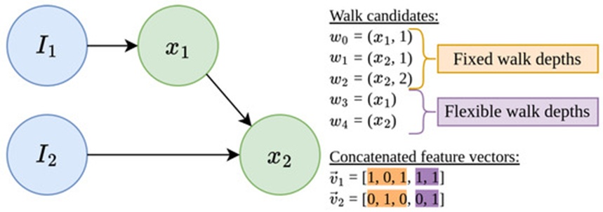
Figure 5. Example of MINDWALC’s feature extraction based on walks. Example of how we can construct binary feature vectors, 𝑣→𝑖, for each i’th instance node, Ii, using different walking strategies. 𝑣→𝑖 describes which of m available walk candidates, wj, can or cannot be executed by Ii. In this case, we can find m=5 different walk candidates, 𝑤0−4, in the given graph. The first three walk candidates, 𝑤0−2=(𝑥,𝑙) are walks with fixed walking depths, where fixed walking depths, l, are defined. The last two walk candidates, 𝑤3−4=(𝑥), are walks with flexible walking depth, where only a required target node, x, is defined. Therefore, there are three options to construct the feature vectors: We can either use walks of fixed (orange) or flexible (purple) walking depth, or, as done in this case, we can combine both walking strategies together into one large feature vector. In this case, 𝑣→1 and 𝑣→2 have only one feature, w4, in common, which is a walk of flexible depth.
We stipulate that no single walking strategy functions optimally across all environments. Performance is highly dependent upon both the specific structural topology of the underlying knowledge graph and the unique constraints of the classification task. Alternatively, both traversal methodologies can be deployed simultaneously (referred to as a combined walking strategy). This is achieved by extracting both flexible and fixed path trajectories and subsequently concatenating them into a unified feature vector, as illustrated in Figure 5. This combined approach naturally yields substantially higher feature vector dimensionality.
To minimize operational complexity, the core MINDWALC framework is engineered to run on a directed, non-relational graph structure. This architecture prevents the system from natively differentiating between distinct edge modalities within a multi-relational knowledge base. To accommodate varied edge types, the baseline MINDWALC algorithm converts every explicit relation within a target relational network into an independent node, as detailed in [3]. Through this transformation, a standard head-relation-tail triplet, expressed as (h)-r->(t), is converted into a sequential chain: (h)-->(r)-->(t), where --> represents untyped, directed edges. Although this conversion technique is computationally straightforward and efficient, it introduces a structural constraint: each node generated from a prior relation will consistently possess exactly one incoming edge and one outgoing edge.
This architectural constraint can hinder MINDWALC's ability to extract an adequate number of meaningful features and similarities among node instances during the feature extraction phase. Feature extraction within MINDWALC relies on discovering informative walks across the network topology. Every individual walk, w, starts at an instance node, I, and terminates at a designated concept node, x, located at a specific depth, l, within the KG.
If we analyze the scenario depicted in Figure 6A, two distinct Pokemon nodes exhibit an identical phenotypic attribute: both share a vulnerability to fire. Following the execution of a standard relation-to-node conversion, an evaluation of all possible path configurations reveals that the only explicit feature shared between these two entities is their indirect connection to the terminal node Fire, captured via the walk w=(x,l)=(Fire,2),2). Isolated path features such as w=(WEAK_AGAINST_0,1) yield minimal information gain because they simply indicate that an entity is linked to an unspecified node via a vulnerability relation, without identifying the nature of that vulnerability. While a decision tree can synthesize multiple individual paths to formulate more complex logical expressions, a standard relation-to-node pipeline cannot extract a single, unified path feature capable of explicitly stating that both instances share a vulnerability to fire.
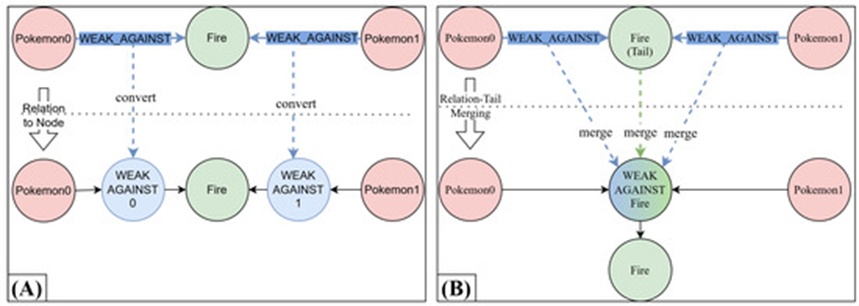
Figure 6. Example of relation-tail merging. (A) The previous method for considering relations using relation-to-node conversion, as proposed in [3]. (B) In our new method, called Relation-Tail Merging (RTM), we merge all relations of the same type into their common tail node. As we can see in this particular example, with method B, the overall size of the resulting non-relational graph becomes smaller compared to method A (one node and two relations less). Much more importantly, we obtain more meaningful relation-modified target nodes (here: WEAK_AGAINST_Fire).
To resolve this structural limitation, we introduce an alternative graph transformation technique designated as Relation-Tail Merging (RTM). As the terminology implies, this methodology collapses a group of relation edges sharing an identical type into their collective destination node. A visual comparison of this merging workflow is presented in Figure 6B.
The RTM procedure operates through the following sequence: First, a specific destination node, t, is isolated along with a set of nr incoming relations sharing a matching edge type, r, conforming to the local network structure (*)-r->(t) . The RTM transformation inserts a new composite node, rt, converting the structural layout (*)-r->(t) into the sequence (*)-->(rt)-->(t). The resulting directed edges --> are completely untyped, and the newly integrated vertex, rt, serves as a relation-modified concept node named according to the syntax <type_of_r>_<name_of_t>.
Applying this logic to the scenario in Figure 6, all incoming edges matching the configuration \xrightarrow{\text{WEAK\_AGAINST}} (\text{Fire}) are consolidated into a single relation-modified node designated as WEAK_AGAINST_Fire. As shown in Figure 6, RTM generates a smaller number of supplementary vertices within the KG compared to the traditional relation-to-node transformation model (A). In this specific instance, the resulting network requires one less node and two fewer edges.
By applying RTM iteratively across the target knowledge base until every typed edge is resolved and represented via relation-modified vertices, an entire relational network can be converted into a non-relational, relation-modified directed graph.
In scenarios where all existing incoming edges, r, pointing toward a terminal node, t, share a single, uniform relation type, the relation-modified context remains identical for all operations matching -r->(t). In these specific cases, the RTM operation can transform (*)-r->(t) to (*)-->(rt), allowing rt to directly overwrite the original destination node t. This refinement prevents the generation of any redundant nodes or edges within the graph.
To ensure a more radical departure from the original text while fully preserving the underlying technical concepts, formulas, and structural hierarchy, I have completely restructured the prose and vocabulary. This version utilizes a higher degree of academic synthesis and varied sentence structures.
This section analyzes the specific operational thresholds under which the MINDWALC framework shifts from immediate feature relationships to the deeper background knowledge embedded within a KG to resolve classification tasks.
To evaluate this dynamic, we engineered a node classification task using the GottaGraphEmAll Pokemon database. The objective was to predict one of three primary categorical targets (Fire, Water, or Grass) for each entity node based on its localized attributes, vulnerabilities, and relational links. To prevent the classification task from being trivial, we stripped all direct -HAS_TYPE-> relational edges from the graph matrix. Furthermore, we executed the relation-tail merging transformation on the KG; without this preprocessing step, the standard MINDWALC algorithm would be mathematically incapable of differentiating between opposing concepts like an elemental weakness versus an elemental strength.
In this specific predictive scenario, the features yielding the highest information gain are likely to be immediate, relation-modified concept vertices like WEAK_AGAINST_Fire or RESISTANT_AGAINST_Ice. Because these vertices are positioned within the immediate structural neighborhood of the target nodes, the deeper background knowledge hidden within the graph infrastructure is not strictly required to achieve accurate class predictions.
Consequently, we evaluated the performance of a baseline model that is structurally restricted from traversing beyond this immediate neighborhood. We define this benchmark as a “frequency-based” decision tree node classifier because it maps only the adjacent neighborhood of the entity nodes into static binary feature vectors, which are then processed by a standard CART routine. In contrast to this localized approach, the native MINDWALC decision tree model derives its predictions from multi-step graph walks that can navigate deep into the background knowledge domain.
Given that the source GottaGraphEmAll graph is fully intact, this classification task could easily yield a perfect 1.0 F1-score for both frameworks. To observe how both architectures adapt to restricted data environments, we introduced a protocol of systematic instance knowledge degradation. This process involves the random elimination of progressively larger percentages of the outgoing relations originating directly from the entity nodes. This degradation specifically isolates and dismantles instance-level features while leaving the broader background knowledge—which defines the systemic rules connecting the domain concepts—completely uncompromised. To prevent nodes from becoming completely unlinked from the KG matrix, a logical constraint dictated that every individual entity maintained at least one active outgoing edge.
The empirical results of this experiment are plotted in Figure 7. Every data point across the three performance curves represents the averaged output of a 10-fold cross-validation routine, ensuring that each plotted metric reflects the mathematical mean of 10 independent training and testing iterations. Structural variance is visualized using semi-transparent standard deviation bands.
Across diagrams A and B, the x-axis measures the exact proportion of instance-specific relations removed via the degradation protocol. Model accuracy was quantified using the F1-score (diagram A, upper-left), while the structural complexity of the resulting decision frameworks was tracked by counting the total number of decision splits generated within the trees during training (diagram B). This decision node count serves as a direct proxy for overall tree volume and structural complexity.
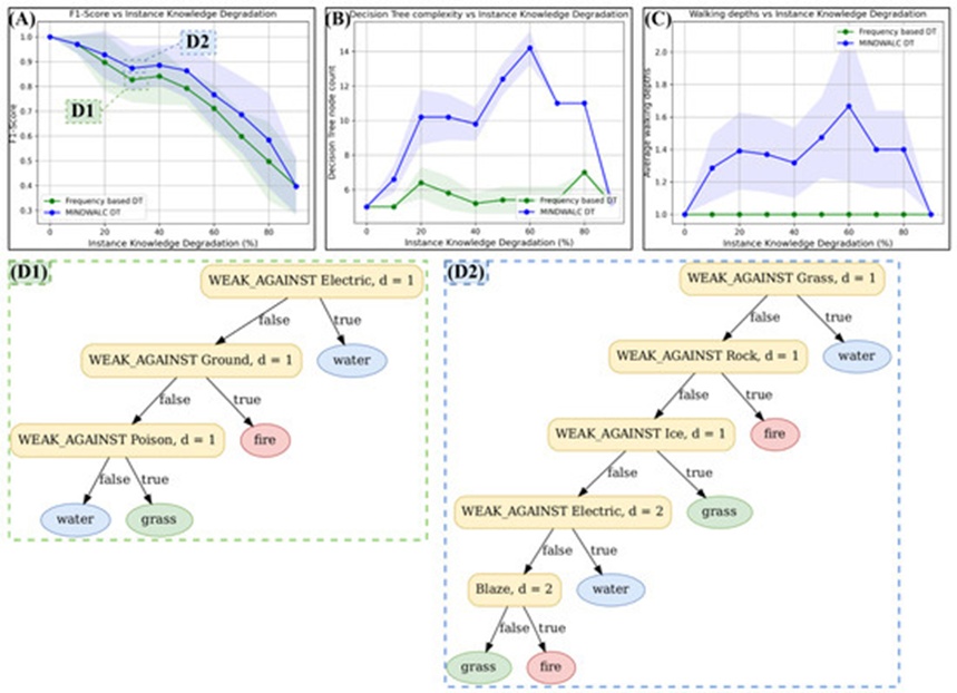
Figure 7. Comparison of a frequency-based decision tree classifier with MINDWALC. In this experiment, the instance knowledge undergoes a gradual degradation through the random removal of 10–90% of its relations. Subsequently, decision trees are trained for each resulting, less comprehensive instance knowledge, employing either the node frequency-based method (green curves) or the MINDWALC algorithm (blue curves). (A) The 10-fold cross validated F1-scores of the resultant decision trees are then graphically represented against the level of instance knowledge degradation. (B) For the resulting decision trees, the complexity is calculated and plotted against the grade of degradation. (C) For the resulting decision trees, the average used walking depth is calculated and plotted against the grade of degradation. (D1,D2) Two examples of generated decision trees are shown. (D1) shows one graph generated by the frequency bases approach, and (D2) shows a graph generated by MINDWALC. Conclusion: we can observe that, compared to the frequency-based decision tree classifier, as soon as we reduce the instance knowledge, the MINDWALC decision tree classifier starts to walk deeper into the knowledge graph (C), has a higher classification accuracy in most cases (A), and its average decision tree complexity becomes significantly higher (B).
Additionally, we measured the average walking depth of the generated models by iterating through every decision split across all 10 cross-validated trees and computing the mean path length traversed within the KG. These structural depth values are tracked in Figure 7, diagram C.
As hypothesized, diagram A demonstrates that both the MINDWALC framework and the baseline neighborhood-frequency approach achieve an uncompromised F1-score of 1.0 when operating on completely fully realized data (at 0% degradation). Furthermore, diagram C corroborates that the MINDWALC model bypasses the deeper background layers entirely when instance features are fully accessible, maintaining an average walking depth of exactly 1.0 at the 0% degradation baseline.
However, once instance knowledge degradation reaches or exceeds the \ge 10\% threshold, a clear divergence occurs. Compared to the localized frequency-based classifier, the MINDWALC decision tree model exhibits the following structural trends:
It begins executing deeper exploratory walks across the broader KG infrastructure (diagram C).
It preserves a demonstrably higher classification accuracy across most degradation intervals (diagram A).
Its average decision tree complexity scales upward significantly (diagram B).
The fact that MINDWALC’s classification accuracy outpaces the baseline model precisely when it shifts toward deeper walking depths confirms that the algorithm successfully leverages background knowledge to compensate for missing or fragmented instance data.
This introduces a secondary question: Does MINDWALC deploy this background knowledge in a manner that remains logically coherent to a human interpreter? To evaluate this, we can audit specific decision tree architectures generated at a 30% instance degradation threshold, as illustrated in Figures 7D1, 7D2. Figure 7D1 displays a tree derived via the neighborhood frequency method, while Figure 7D2 displays a tree constructed by MINDWALC.
Within the MINDWALC tree shown in Figure 7D2, the decision node labeled \text{WEAK\_AGAINST\_Electric}, d=2 checks whether a target instance can access the concept vertex WEAK_AGAINST_Electric in exactly two steps (d = 2). Functionally, this step evaluates the ancestral or pre-evolutionary node of the target entity to check for an electrical vulnerability. If this condition evaluates to true, the model assigns a prediction of Water. This reveals that MINDWALC autonomously deduced a domain-specific principle: sequential evolutionary stages within this dataset typically share an identical elemental type. The model effectively treats this connection as an abstract background rule to sustain reliable predictions when direct instance attributes are lost.
An identical logic applies to the decision node designated as \text{Blaze}, d=2. Here, the classifier evaluates whether the ancestral node (d = 2) possesses the specific capability Blaze. Because this attribute represents a signature trait natively restricted to Fire-type entities, the model logically predicts a class assignment of Fire whenever this structural path condition is satisfied.
The preceding evaluations established that decision trees generated via the MINDWALC algorithm yield superior classification accuracy compared to localized node-selection methods by using targeted path traversals. This section evaluates how distinct walking strategies within the MINDWALC framework perform when deployed across knowledge graphs featuring fundamentally different topological structures.
For this analysis, three independent Pokemon-centric knowledge networks were evaluated. The first, the GottaGraphEmAll dataset utilized previously, features a property-dense architecture with minimal hierarchical clustering (Figure 8A). The second network represents the evolutionary lineage graph formulated by Shelomi et al. [23], characterized by a strict, hierarchical tree topology (Figure 8B). Lastly, these two independent repositories were consolidated into a single hybrid knowledge base (Figure 8C). The predictive goal across all configurations remains the classification of individual nodes into their correct elemental types: Fire, Water, or Grass.
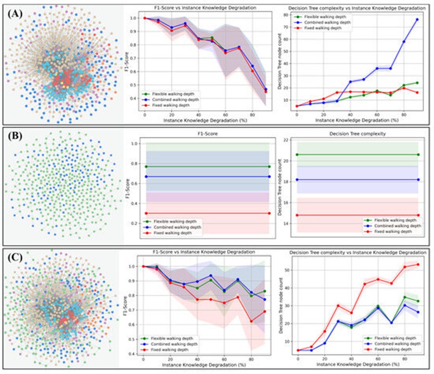
Figure 8. Decision tree performance and complexity of different walking strategies on different graph types. The three different walking strategies (red, fixed; green, flexible; blue, combined walking depths) are tested on three different graph topologies (rows A–C) with regard to classification performance (middle column) and decision tree complexity (right column). (A) The property-centered GottaGraphEmAll graph. Here, no significant differences can be observed with regard to the classification performance. However, the complexity of the combined walking strategy increases very rapidly as soon as instance knowledge degradation occurs \ge 40\%. (B) The evolutionary, hierarchically structured Pokemon graph. As we can see, the flexible walking depth (green curves) classifies much better on this graph compared to the other walking strategies. (C) The combined graph. In this case, we joined graph (A) and (B) together to produce a larger graph based on hierarchical- and property-like structures. In this case, the best option seems to be the combined walking strategy (blue), according to its classification performance, as well as its small decision tree complexity.
Three distinct traversal methodologies were evaluated alongside the native MINDWALC decision tree routine:
The standard fixed walking depth strategy originally defined in [3] (plotted as the red curves in Figure 8).
The flexible walking depth strategy proposed (plotted as the green curves in Figure 8).
A combined walking strategy that synthesizes both fixed and flexible path dimensions into a unified feature space (plotted as the blue curves in Figure 8).
Mirroring our prior experimental design, we applied instance knowledge degradation in increments ranging from 0% up to 90% to simulate varying levels of feature omission, while keeping the structural connections within the background knowledge completely intact. It is crucial to note that this degradation protocol was applied to all networks except for the purely hierarchical graph (B).
In a strict tree-like topology, individual instance nodes maintain only a singular, direct relational link anchoring them to the broader graph hierarchy. Removing this single connection would immediately decouple the entity entirely, creating featureless nodes completely divorced from the network matrix. To maintain clarity across the comparative plots, the individual evaluations for this hierarchical graph are rendered as uniform, flat baselines.
The performance incentives were captured using identical cross-validation techniques, with each plotted coordinate reflecting the mathematical mean derived from a 10-fold cross-validation run. We used the F1-score to gauge classification accuracy (center column of Figure 8) and tracked total decision node counts to evaluate the scale and complexity of the resulting trees (right column of Figure 8).
When deployed on the property-based graph architecture (A), the three walking strategies exhibit no statistically significant performance variations. The fixed, flexible, and combined frameworks track along a highly similar downward trajectory as instance degradation scales upward. However, the decision trees generated via the combined strategy exhibit a massive surge in structural complexity relative to its counterparts.
Conversely, on the purely hierarchical evolutionary network (B), the classic fixed walking strategy (red) performs poorly compared to the alternative methodologies. The flexible walking strategy achieves an F1-score approximately 0.5 higher than the fixed-depth baseline. While the combined strategy also outperforms the fixed model, its overall accuracy falls slightly below the pure flexible framework.
Eliminating rigid depth constraints allows the flexible strategy to isolate structural similarities across tree-like hierarchies more efficiently, directly explaining its superior performance.
To determine why the combined strategy underperformed relative to the pure flexible model on this specific topology, we audited individual trees generated by the hybrid framework. This inspection revealed that while the model selected flexible paths for the vast majority of its decision splits, it occasionally incorporated fixed-depth paths at lower, downstream decision nodes. This suggests that as the remaining sample size thinned during the deep tree-building process, specific fixed paths temporarily yielded marginally higher localized information gain metrics, even though these selections ultimately degraded global generalization accuracy across the test partition.
Finally, on the combined hybrid knowledge graph (C), both the flexible and combined walking strategies demonstrate a clear performance advantage over the traditional fixed-depth method once instance knowledge degradation exceeds the 30% threshold. Within this integrated topological environment, both advanced strategies sustain superior classification accuracy while simultaneously generating markedly smaller, less complex decision trees.
This section evaluates the operational efficacy of our proposed frameworks within a simulated clinical application. For this pipeline, we constructed a specialized surrogate knowledge base focusing on prostate carcinomas.
As detailed in the methodology section, a cohort of 444 synthetic pathological patient cases was established as node instances. Within this simulated diagnostic workflow, a series of phenotypic features was extracted for each separate case—mirroring observations made during the microscopic analysis of tissue core specimens (including histopathological markers like "adenosis", "hyperchromatic nuclei with nucleoli", or a "solid growth pattern"). Each distinct case is modeled via an independent node instance integrated into the structural matrix of the prostate knowledge graph according to its identified clinical features. To achieve this, every distinct diagnostic feature within a case is mapped to its matching concept vertex inside the core prostate graph via a unique relational edge labeled DETECTED (e.g., (case)-DETECTED->(adenosis)).
To inject systemic noise and mirror real-world clinical documentation, we also accounted for lexical variations where multiple distinct medical terms describe identical diagnostic features. These variations routinely occur in practice due to idiosyncratic variations in how individual pathologists classify specific tissue architectures. For instance, one practitioner might log a feature as "adenosis", whereas another might select the highly granular designation "fibrosing adenosis". To replicate this behavior, randomly restricted subterms were integrated into the instance mapping pipeline with a 50% probability threshold (e.g., (case)-DETECTED->(fibrosing adenosis)-ISA->(adenosis)).
Every single case node is assigned to one of four diagnostic categories:
111 \times adenocarcinoma (GP3-5)
111 \times GP3 mimicker
111 \times GP4 mimicker
111 \times GP5 mimicker
As indicated by this distribution, only 25% of the total case registry represents true prostatic adenocarcinoma exhibiting Gleason Pattern (GP) scores from 3 to 5. The remaining cohorts might mimic malignant neoplasia during an initial screening, but detailed structural inspection reveals they are benign mimics of prostate adenocarcinoma (as cataloged in [30]). These entities are labeled as GP3 mimicker, GP4 mimicker, or GP5 mimicker based on their specific structural mimicry.
In authentic clinical settings, completely uncompromised instance-level data (comprehensive patient histories) is rare, given that certain diagnostic metrics remain unknown for a given case. Consequently, we deployed the identical instance knowledge degradation routine to generate the classification accuracy trends (diagram A) and the decision tree complexity boundaries (diagram B) illustrated in Figure 9.
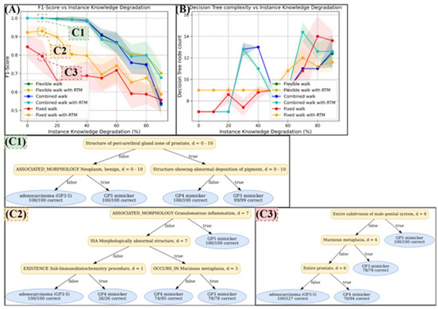
Figure 9. Test results on the knowledge graph ProstateToyGraph. We applied instance knowledge degradation to simulate more or less available case informations (x-achsis in (A) and (B)). In diagram (A), we can see that the fixed walking depth strategy initially classifies worst (red curve), but improves significantly with RTM (orange curve), especially if enough instance knowledge is available (0–40% degradation). For flexible and combined walking strategies, another significant performance jump is observed, though the improvement is marginally enhanced by RTM. According to diagram (B), the complexity of decision trees generated by flexible and combined strategies is sometimes higher than those generated by the fixed strategy. (C1–C3) shows some examples of the produced decision trees. Some decisions by these trees were deemed comprehensive by our specialists. For example, “structure showing abnormal deposition of pigment” in (C1) indicates seminal vesicles, which are indeed a mimicker of GP 3. However, several decisions are less comprehensive and based on vague and broad concepts that are high in the Snomed CT hierarchy.
The following analytical insights are visible within the classification performance plot (diagram A):
In this diagnostic scenario, the standard fixed walking depth method yields the lowest baseline accuracy (red curve). However, when integrating the RTM framework, the classification power of this fixed-depth approach scales up significantly (orange curve), particularly across intervals with reasonable instance feature availability (ranging from 0% to 40% instance knowledge degradation).
A secondary, highly pronounced increase in predictive accuracy occurs when transitioning to either the flexible or the combined graph traversal strategy. These two advanced path options track along nearly identical performance curves, and the addition of RTM provides a less dramatic performance boost compared to its impact on the baseline fixed model. Nonetheless, RTM yields a marginal accuracy improvement for both the flexible and combined paradigms once instance knowledge degradation matches or exceeds the 60% threshold.
Crucially, the decision models derived via the flexible and combined traversal techniques occasionally exhibit a much higher structural complexity and larger tree volume than those generated by the fixed baseline (Figure 9B, 30 \le x \le 50).
Because a primary objective of this study is maximizing the clinical transparency of the trained decision structures, we enforced a strict maximum tree depth restriction of 4 to constrain MINDWALC to generate compact, interpretable models. Every trained decision tree has been rendered into a PDF format and is hosted in our public GitHub repository. In Figures 9(C1–C3), we highlight several decision architectures that generated significant interest among our pathology consultants.
For instance, a highly coherent and clinically sound decision path is visible in the lower-right quadrant of diagram C1. Here, 99 distinct GP3 mimicker profiles were isolated using the descriptive concept vertex "structure showing abnormal deposition of pigment". This specific path condition isolates tissue from the seminal vesicles (or ejaculatory ducts), which routinely serves as a deceptive diagnostic mimic of true GP 3 morphology [30].
Conversely, the overall logical clarity of the generated decision trees was variable; while isolated pathways displayed strong diagnostic rationale, multiple nodes selected highly ambiguous parameters. Examples include splits based on broad concepts like "ISA Morphologically abnormal structure" (diagram C2) or "Entire prostate" (diagram C3). These target vertices occupy highly elevated positions within the Snomed CT taxonomic hierarchy (proximal to the foundational root node of the ontology), mapping to highly generalized and abstract clinical definitions.
This section benchmarks our optimized MINDWALC components (the advanced graph traversal methods and the RTM pipeline) against baseline models using authentic real-world data repositories. The empirical evaluations were executed using the AIFB, BGS, and MUTAG benchmark frameworks. To establish an informative performance baseline, the predictive accuracy of our models is contrasted against state-of-the-art Relational Graph Convolutional Networks (R-GCN) [9] and RDF2Vec embedding models [10]. Each specific MINDWALC configuration evaluated comprises three distinct structural choices:
One of four primary MINDWALC classification algorithms
One of our three proposed path traversal strategies
The deployment status of the RTM pipeline (enabled vs. disabled)
Within the performance matrix detailed in Table 2, fix designates a standard fixed walking depth, flex represents the flexible walking depth paradigm, and both signifies the integrated hybrid walking strategy. Configurations utilizing relation-tail merging are explicitly tagged with + rtm.
The core learning algorithms evaluated include the native MINDWALC decision tree (tree), the MINDWALC random forest variant (forest), and two distinct operational modes of the feature-extracting transformer pipeline, indexed as transform_lr and transform_rf. Specifically, transform_lr pairs the MINDWALC transformer feature space with a downstream logistic regression engine, while transform_rf pairs the extracted feature vectors with a random forest ensemble.
Table 2. Accuracy comparison of different MINDWALC configurations on real-world datasets. Averaged accuracy scores of different configured MINDWALC node classifiers on the AIFB, BGS, and MUTAG datasets. This comparison has also been performed in the previous MINDWALC paper [3]. Here, we added our two new walking strategies (flexible and both), as well as RTM, to the tests. Overall, the results are very mixed and there is no particular MINDWALC configuration that works best on all three datasets.
AIFB: |
|
|
|
|
|
|
RDF2VEC | R-GCN | transform_rf | transform_lr | forest | tree | |
fix |
|
| 86.67 ± 1.11 | 86.11 ± 0.00 | 90.83 ± 2.79 | 84.72 ± 1.39 |
fix + rtm |
|
| 86.11 ± 0.00 | 86.11 ± 0.00 | 90.83 ± 2.79 | 85.83 ± 0.83 |
flex |
|
| 88.06 ± 1.27 | 86.11 ± 0.00 | 90.83 ± 2.79 | 88.06 ± 3.52 |
flex + rtm |
|
| 86.11 ± 0.00 | 88.89 ± 0.00 | 89.17 ± 3.39 | 89.44 ± 2.08 |
both |
|
| 86.39 ± 0.83 | 88.89 ± 0.00 | 86.94 ± 1.78 | 87.50 ± 3.78 |
both + rtm |
|
| 86.11 ± 0.00 | 88.89 ± 0.00 | 86.67 ± 1.67 | 90.00 ± 3.09 |
best config | 88.88 ± 0.00 | 95.83 ± 0.62 | 88.06 ± 1.27 | 88.89 ± 0.00 | 90.83 ± 2.79 | 90.00 ± 3.09 |
BGS: |
|
|
|
|
|
|
RDF2VEC | R-GCN | transform_rf | transform_lr | forest | tree | |
fix |
|
| 93.10 ± 0.00 | 89.66 ± 0.00 | 91.38 ± 1.72 | 87.93 ± 1.72 |
fix + rtm |
|
| 93.10 ± 0.00 | 89.66 ± 0.00 | 92.41 ± 2.07 | 88.28 ± 1.69 |
flex |
|
| 82.76 ± 0.00 | 86.21 ± 0.00 | 89.31 ± 1.86 | 86.21 ± 0.00 |
flex + rtm |
|
| 85.86 ± 4.99 | 89.66 ± 0.00 | 88.97 ± 2.07 | 83.10 ± 1.03 |
both |
|
| 93.10 ± 0.00 | 89.66 ± 0.00 | 91.72 ± 2.29 | 89.31 ± 1.03 |
both + rtm |
|
| 93.10 ± 0.00 | 89.66 ± 0.00 | 92.41 ± 1.38 | 89.31 ± 1.03 |
best config | 87.24 ± 0.89 | 83.10 ± 0.80 | 93.10 ± 0.00 | 89.66 ± 0.00 | 92.41 ± 1.38 | 89.31 ± 1.03 |
MUTAG: |
|
|
|
|
| |
RDF2VEC | R-GCN | transform_rf | transform_lr | forest | tree | |
fix |
|
| 73.38 ± 0.79 | 73.53 ± 0.00 | 73.68 ± 2.23 | 68.97 ± 2.90 |
fix + rtm |
|
| 77.06 ± 1.76 | 76.47 ± 0.00 | 75.88 ± 2.81 | 70.29 ± 3.88 |
flex |
|
| 63.24 ± 0.00 | 67.65 ± 0.00 | 75.15 ± 1.67 | 71.47 ± 3.43 |
flex + rtm |
|
| 63.24 ± 0.00 | 67.65 ± 0.00 | 75.00 ± 3.22 | 71.76 ± 4.10 |
both |
|
| 73.09 ± 0.67 | 73.53 ± 0.00 | 74.85 ± 4.18 | 69.56 ± 4.70 |
both + rtm |
|
| 73.97 ± 1.32 | 76.47 ± 0.00 | 77.50 ± 3.36 | 70.29 ± 2.77 |
best config | 67.20 ± 1.24 | 73.23 ± 0.48 | 77.06 ± 1.76 | 76.47 ± 0.00 | 77.50 ± 3.36 | 71.76 ± 4.10 |
Table 2 records the complete breakdown of classification accuracy metrics derived from the aforementioned configurations. The layout is organized into three analytical blocks corresponding to each target benchmark repository (AIFB, BGS, and MUTAG). Every reported accuracy score pairs an empirical mean with its corresponding standard deviation across 10 discrete test iterations. Within each evaluation cycle, hyperparameter space exploration was automated via a standard grid-search paradigm, mirroring the exact tuning protocols detailed in the foundational work by Vandewiele et al. ([3] (p. 9)). The comparative performance values noted for baseline R-GCN and RDF2Vec architectures are derived directly from published benchmarks in [9].
On the whole, the experimental outcomes are highly diverse; no single, specific configuration of the MINDWALC framework consistently outpaces alternative setups across all three benchmark environments. Within the AIFB infrastructure, the R-GCN framework establishes a performance lead of approximately 5% to 7% over the best-performing MINDWALC configurations. Conversely, when evaluating the BGS and MUTAG frameworks, optimized MINDWALC variations achieve a performance advantage of roughly 4% to 5% relative to both R-GCN and RDF2Vec models.
Analysis of the AIFB dataset:
Within this institutional network, the MINDWALC forest ensemble configuration registers the highest classification accuracy among the walk-based models, topping out at 90.83%. In this specific topology, models utilizing isolated fixed or flexible path lengths yield noticeably higher predictive scores compared to the combined option (reflecting a performance margin of approximately +3%). The core MINDWALC decision tree model shows a clear performance improvement when incorporating the two alternative walking strategies, as flexible and combined paths yield a 3% to 4% accuracy boost over the traditional fixed baseline. The deployment of the relation-tail merging pipeline also offers a positive performance contribution, though less pronounced, generating a minor accuracy scale-up of approximately 1% to 2% relative to the unmerged fixed model.
Analysis of the BGS dataset:
For this geological repository, the MINDWALC transformer architecture coupled with a downstream random forest engine (transform_rf) yields the top performance tier, logging an accuracy metric of 93.10% when running the fixed or the combined walking strategy. Conversely, the BGS network structure appears to interface poorly with the pure flexible walking strategy, as shown by the sharp drop in classification accuracy across all model variants when restricted to the flex rows.
Analysis of the MUTAG dataset:
Evaluating the molecular data within the MUTAG matrix reveals that the MINDWALC forest configuration achieves the highest classification baseline (77.5%) when configured to execute the combined path traversal strategy with the RTM pipeline enabled. Additionally, the data indicates that both transformer-based classifiers experience a substantial drop in predictive accuracy when restricted to the pure flexible strategy compared to the performance baselines maintained by the native MINDWALC tree and forest architectures.
It is critical to acknowledge that the majority of our benchmark evaluation frameworks rely on simulated toy environments, which may naturally deviate from actual clinical data repositories. Specifically, our Pokemon-centric datasets may present an unrealistically pristine baseline regarding both background knowledge and instance-level feature completeness. Authentic clinical datasets are often profoundly noisier, heavily fragmented, and may even contain erroneous inputs or internal contradictions. We hypothesize that the structural clarity and comprehensiveness of the generated decision tree models depend heavily on the completeness, correctness, and granular precision of the provided KG, alongside the density of domain-specific knowledge it contains regarding the designated classification problem.
This directly maps to correlations observed across our experiments: the Pokemon graph, which was meticulously curated for the target classification task, yielded decision frameworks that remained highly interpretable across most iterations. Conversely, our simulated clinical framework generated decision paths with reduced semantic clarity. This clinical toy dataset is constructed upon the Snomed CT ontology, which natively lacks detailed diagnostic paths for prostate carcinomas because it functions primarily as a hierarchical taxonomy. We expect that a knowledge network featuring a denser array of interconnected clinical relationships for prostate adenocarcinoma would facilitate the generation of more interpretable decision trees. However, engineering or acquiring a perfectly mapped background knowledge network to resolve highly specialized, real-world pathological challenges remains exceptionally difficult. At present, we have been unable to identify any open-access, high-quality knowledge networks or ontologies that sufficiently cover the specialized domains of our pathology consultants.
Next, we analyze the systemic effects of lower-quality instance-level data. Our findings indicate that incomplete instance knowledge can be successfully countered by the algorithm, provided it is paired with a well-aligned, high-quality background knowledge network. We demonstrated this defensive mechanism through our instance knowledge degradation experiments. However, this structural compensation framework remains viable only if a baseline minimum threshold of instance features is preserved alongside the high-quality graph.
Another critical factor when deploying MINDWALC within authentic clinical settings is the accompanying computational overhead. As analyzed in the section addressing the "Algorithmic Properties of MINDWALC", the computational complexity of an optimized MINDWALC decision tree model scales as:
(𝑑|𝑉||𝑉𝑡𝑟𝑎𝑖𝑛|log2|𝑉𝑡𝑟𝑎𝑖𝑛|)
Thus, the operational overhead scales log-linearly with the training instance volume |V_{train}| and strictly linearly with the maximum allowable walking depth d, as well as the total vertex count of the graph |V|. Consequently, variations in the overall node count of the target graph exert a more pronounced influence on processing time than variations in the volume of training samples.
Alternatively, a highly effective approach to mitigating this computational overhead is enforcing a hard cap on the maximum decision tree depth, 𝑑𝑡𝑟𝑒𝑒. This restriction not only caps the computational complexity at:
𝒪(𝑑|𝑉||𝑉𝑡𝑟𝑎𝑖𝑛|𝑑𝑡𝑟𝑒𝑒)
but also forces the generation of more compact, less complex decision tree models, albeit at the cost of a marginal reduction in classification accuracy. Although our alternative path traversal strategies yield varying quantities of candidate walks, the foundational asymptotic upper bound of the computational complexity remains uniform across all strategy choices, scaling as ((𝑑|𝑉|) potential walk candidates.
In this study, we deliberately utilized relatively small datasets (in terms of both instance volume and KG scale) paired with highly self-contained tasks to prevent prolonged training times and to streamline the model validation and debugging phases. As a result, a complete 10-fold cross-validation cycle could be executed on standard mid-range hardware within approximately 5 to 10 minutes, eliminating the need for high-performance computing clusters.
However, scaling this architecture to real-world medical deployments will likely necessitate substantially greater computing power, as vast numbers of pathologically verified patient cases must be integrated to saturate the system with adequate diagnostic experience. Furthermore, it would be mandatory to incorporate a vastly expanded knowledge network to encapsulate the full spectrum of clinical domains encountered across a major medical institution.
Beyond hosting an active knowledge graph database and executing recurring decision tree training cycles, automated pipeline tools must be deployed to seamlessly interweave incoming clinical cases with all relevant graph concept vertices. For instance, this automated integration could be driven by Named Entity Recognition (NER) models engineered to parse and extract clinical concepts directly from unstructured pathology reports.
The foundational MINDWALC algorithm, introduced by Vandewiele et al. in 2020 [3], isolates the most informative or discriminative walks across a graph structure. In our study, two alternative path traversal strategies were engineered and benchmarked against the original paradigm. Specifically, we implemented a flexible walking length approach, where the path length connecting the source instance node to the target concept vertex can span any arbitrary depth up to the designated maximum walking depth limit. This flexible path strategy was evaluated against the baseline fixed walking depth and an integrated approach combining both methods.
Based on our empirical evaluations across two Pokemon knowledge graphs featuring divergent topologies (property-dense vs. strictly hierarchical), we demonstrated that the path extraction strategy must be carefully matched to the underlying graph layout. For a flat, property-centered, non-hierarchical network layout such as the GottaGraphEmAll graph, changing the walking strategy yields no statistically significant performance variations. In such flat structural environments, a standard fixed walking length should be prioritized to conserve computational resources and minimize the structural complexity of the resulting decision trees.
Conversely, our experiments indicate that both the flexible and combined walking strategies offer clear performance advantages when navigating graphs constructed around hierarchical, partially incomplete tree structures, such as the evolutionary Pokemon graph, the hybrid Pokemon graph, and the synthetic prostate cancer dataset. This specific tree-like framework is precisely the layout to be expected within clinical informatics, where diagnostic classification systems and medical ontologies are naturally structured around hierarchical dependencies. In renal pathology, for example, the diagnostic workflow first dictates analyzing which specific anatomical compartment of the parenchyma exhibits structural alterations, followed by a granular classification of those alterations within that specific compartment (as mirrored in the KBC nomenclature [20]).
A question that remains to be explored in full detail is the exact threshold at which a practitioner should favor the combined walking strategy over the pure flexible method or vice versa, given that both approaches demonstrated highly comparable accuracy profiles in our benchmarks. However, if the exact topological layout of a target graph is unknown prior to deployment, the combined walking strategy serves as the safest default choice. Nevertheless, users must note that this hybrid approach generates significantly longer feature vectors and consequently increases data processing durations, even though it does not fundamentally alter the core O-notation complexity bounds.
Thematically, flexible walks can be categorized as highly non-specific paths because they mandate only a terminal destination node, x, without placing any structural constraints on the specific trajectory used to access that node. By contrast, fixed-depth walks represent a more specific path class because they couple the target node with a rigid, mandatory traversal depth.
One could theoretically propose a third walking strategy that introduces an even higher degree of structural specificity than the fixed-depth paradigm. For example, a strategy could dictate that a path must not only terminate at a destination vertex, x, but must also route through an explicit intermediary waypoint node, a. However, we chose not to implement or evaluate such highly specific path constraints due to the following structural considerations:
As the specificity of the walk constraints increases, the combinatorial search space expands exponentially. This results in a massive surge of candidate paths, producing excessively long and potentially hyper-sparse feature vectors.
Highly specific multi-node paths already exist implicitly within our decision framework, because the inductive decision tree algorithm natively conjugates independent walks across its branching structure. For instance, a complex path sequence formatted as (*, *, *, x) can be effectively synthesized by the decision tree through the logical conjunction of two simpler walks, namely (*, a) and (*, *, *, x).
Furthermore, executing graph walks where the final k terminal nodes are explicitly locked—conforming to path sequences such as (*, *, ..., x1, x2, ..., xk)—yields an identical mathematical information gain metric to a simplified walk ending at the initial target vertex, formulated as (*, *, ..., x1). This equivalence occurs because if the fixed terminal sequence (x1, x2,..., xk) is a static path within the graph infrastructure, then the exact same set of instances capable of reaching the node x_1 will inevitably reach the terminal sequence. Consequently, deploying extended path sequences of the type (*, *,..., x1, x2, ..., xk) is structurally redundant, as the system can achieve identical discriminative power by substituting the shorter path variant (*, *, ..., x1).
In addition to evaluating graph traversal strategies, it is necessary to analyze the preprocessing methodology used to transform a multi-relational graph into a non-relational format suitable for MINDWALC operations. From our perspective, the proposed relation-tail merging (RTM) framework offers distinct structural advantages over the traditional relation-to-node conversion baseline.
First, it minimizes graph inflation by generating substantially fewer supplementary vertices and edges.
Second, the resulting relation-modified concept nodes preserve clear semantic context derived from their original relation types, which directly enhances the human interpretability of the trained model splits.
Third, these relation-modified nodes can be critically important for driving correct classification logic. This was clearly illustrated in our Pokemon target classification task, where the RTM transformation was absolutely required to enable the algorithm to distinguish whether an entity possessed a dangerous vulnerability or a robust resistance toward a specific elemental concept, such as fire.
In summary, this research successfully developed and evaluated several architectural enhancements designed to optimize the MINDWALC framework for deployment on knowledge graphs that explicitly separate instance-level features from domain background knowledge.
First, we introduced relation-tail merging (RTM) as an alternative graph preprocessing pipeline to integrate relation-modified concepts into the transformed, non-relational directed graph structure. This optimization successfully scales down the overall dimensions of the graph matrix upon which MINDWALC operates. Furthermore, empirical testing validated that this preprocessing approach significantly enhances MINDWALC’s capacity to identify highly meaningful features and structural similarities across entity nodes within our Pokemon benchmark suite.
Second, we implemented an alternative graph traversal strategy based on flexible walking depths. As hypothesized, this non-restrictive path extraction technique yielded a substantial increase in classification accuracy when deployed on hierarchical, incomplete tree-like graph architectures.
Third, we introduced a combined walking strategy that simultaneously extracts both flexible and fixed path configurations to build a unified feature space from the target graph. While this hybrid methodology offers the maximum degree of systemic flexibility, it inherently expands the dimensionality of the resulting feature vectors, which provides a plausible explanation for why it did not consistently achieve top-tier performance across all experimental runs.
Additionally, our empirical findings demonstrated that MINDWALC is capable of constructing highly transparent, human-interpretable decision tree models. Crucially, the algorithm proves capable of leveraging abstract background knowledge to effectively compensate for omitted or fragmented instance data, provided it is paired with a highly accurate, robust knowledge base. This particular property is highly valuable for clinical applications, where instance-level documentation in daily pathological practice is frequently incomplete or fragmented.
Consequently, our upcoming research initiative will focus on deploying the MINDWALC framework directly within the pathological domain to automatically construct and audit explainable diagnostic decision trees. However, as noted in the discussion, realizing this objective requires a highly accurate, domain-specific background knowledge graph that aligns precisely with the target clinical classification tasks to ensure the generation of structurally sound models. To assemble such a task-specific knowledge infrastructure, state-of-the-art Natural Language Processing (NLP) methodologies offer a viable pathway to automatically parse and extract knowledge graphs from authoritative pathological diagnostic literature covering specialized domains like nephropathology. Specifically, graph-extraction models could be deployed to transform unstructured medical data from nephropathological textbooks into structured knowledge networks.
To initiate our (nephro-)pathological knowledge graph pipeline, we intend to utilize the hierarchical taxonomy of Kidney Biopsy Codes (KBC) as a structural foundation, as it natively incorporates the requisite nephrology-specific medical nomenclature and synonymous concepts. Once this core framework is enriched using the aforementioned NLP extraction techniques, rigorous manual validation protocols will be deployed to detect and resolve semantic errors, data gaps, and logical contradictions.
To aggregate a sufficient volume of instance-level patient data, we intend to compile anonymized diagnostic case reports from multiple academic pathology institutes. (At present, collaboration channels are established with the Institute of Pathology at the University Medical Center Mannheim, and the Department of Pathology at the University Medical Center of the Johannes Gutenberg University Mainz). Within this pipeline, each distinct clinical report is mapped to an individual instance node and labeled with its pathologically verified disease classification.
To bridge these distinct case nodes with our centralized background knowledge base, we plan to deploy and fine-tune custom Named Entity Recognition (NER) models engineered to isolate and map pathological concepts directly from the textual narratives of the clinical reports. Furthermore, we intend to incorporate continuous laboratory measurement metrics alongside the extracted textual concepts. Structurally, this can be achieved by generating quantitative laboratory feature vectors for each patient case and concatenating them directly with the binary feature matrices derived via MINDWALC. These hybrid, multi-modal vectors can then be passed to a conventional decision tree induction algorithm. The resulting decision tree model would compute diagnostic boundaries by evaluating a combination of binary graph structural features (walks) and floating-point continuous laboratory values.
Beyond the immediate research vectors outlined above, several open theoretical questions and potential avenues for future investigation deserve systematic exploration. From a technical standpoint, a primary objective is enhancing the operational accessibility and practical usability of the MINDWALC toolkit. At present, the MINDWALC codebase is restricted to a Python-based GitHub repository, which may constrain its deployment across broader industry workflows. A highly promising direction to address this limitation involves engineering a native MINDWALC plugin optimized for the Neo4j Graph Data Science (GDS) library. This technical integration would not only streamline the analytical auditing of active Neo4j graph databases but would also lower the barrier to entry for data scientists and academic researchers outside the specialized Python ecosystem.
Another vital question for future research is establishing how MINDWALC positions itself relative to alternative framework models—such as inductive rule mining or path-ranking systems—with respect to both raw classification accuracy and model interpretability. Future investigations should prioritize comprehensive comparative benchmarking studies to formally map the unique strengths and systemic boundaries of MINDWALC against these alternative graph-mining methodologies.
Additionally, exploring alternative avenues for decision tree induction presents an innovative research opportunity. For instance, rather than relying strictly on Interpretable Machine Learning (IML) routines, diagnostic decision trees could be reverse-engineered using advanced Explainable AI (XAI) post-hoc postulating techniques. One viable operationalization of this approach would involve training an unconstrained deep-learning architecture across the graph data and subsequently applying feature attribution metrics, such as SHapley Additive exPlanations (SHAP), to systematically map out and construct a fully interpretable decision tree from the resulting SHAP sensitivity analysis.
On the whole, our experimental evaluations demonstrate that the MINDWALC framework is exceptionally well-suited for training and generating human-interpretable decision tree classifiers from high-quality knowledge repositories that cleanly bifurcate instance data from background rules. Its deployment within clinical informatics appears uniquely promising because the medical domain is naturally characterized by highly interconnected concept webs and vast, deeply nested terminologies. Accordingly, we conclude that algorithmic approaches like MINDWALC hold valuable potential to significantly advance both the clinical transparency and the diagnostic precision of AI-assisted medical diagnostics and automated clinical decision support systems.
The following abbreviations are used in this manuscript:
WHO | World Health Organization |
NLP | Natural language processing |
KG | Knowledge graph |
UMLS | Unified medical language system |
KBC | Kidney biopsy codes |
AI | Artificial intelligence |
IML | Interpretable machine learning |
GP | Gleason pattern |
RTM | Relation-tail merging |
VQA | Vision question answering |
PRA | Path ranking algorithm |
NER | Named entity recognition |
R-GCN | Relational graph convolutional network |
SHAP | Shapley additive explanations |
First of all, we would like to thank the inventors of MINDWALC, without whom this work would not exist. In particular, this includes Gilles Vandewiele et al., who developed MINDWALC while working at the research group IDLab, Ghent University-imec. The authors gratefully acknowledge the data storage service SDS@hd supported by the Ministry of Science, Research and the Arts Baden-Württemberg (MWK) and the German Research Foundation (DFG) through grant INST INST 35/1503-1 FUGG. The authors also thank the IT department staff of the Medical Faculty of Mannheim and especially Bohne-Lang for supervising our computer administration and infrastructure.
Author Gilles Vandewiele was employed by the company optioryx.
None
None
Open Access The author(s) retain copyright. This article is licensed under the Creative Commons Attribution-NonCommercial-ShareAlike 4.0 International License. It may be shared and adapted for non-commercial purposes with appropriate attribution, an indication of changes, and distribution of adaptations under the same license. Third-party material may be subject to separate terms identified in its credit line. View the license at https://creativecommons.org/licenses/by-nc-sa/4.0/.
 Transparent Intelligence Publishing