Global emergency departments and urgent care facilities regularly experience prolonged waiting periods that surpass patient expectations, primarily driven by unexpected spikes in patient volumes. The resulting delays caused by insufficient staffing during these high-demand intervals have been associated with detrimental clinical consequences. Prior investigations into predicting patient volumes have predominantly relied on traditional statistical approaches. Furthermore, these efforts have mainly focused on short-range predictions, which offer minimal utility for the long-term scheduling of medical staff. This paper contributes to a growing domain of research aimed at investigating the capacity of machine learning frameworks to produce precise patient volume projections. Utilizing a decade's worth of data from two major urgent care centers, this study constructs long-range patient flow predictions extending up to one quarter in advance by evaluating a selection of modern, high-performing algorithms. A unique aspect of this research is the integration of eXplainable Artificial Intelligence (XAI) frameworks, specifically LIME and Shapley, to conduct a comprehensive assessment of internal model dynamics that are typically obscured. These diagnostic instruments allowed us to examine how effectively the predictive frameworks adjusted to volatile demand shifts induced by COVID-19 pandemic lockdowns, while also determining the most significant predictor variables to gain deep operational insights. The empirical findings indicate that an innovative ensemble combining gradient boosting techniques with advanced univariate frameworks like Prophet yielded the most precise and dependable performance overall. On average, this methodology produced a 16%–30% improvement over the current internal forecasting techniques utilized for predicting daily patient volumes 90 days into the future.
Urgent Care Clinics (UCCs) and Emergency Departments (EDs) offer continuous, 24-hour medical interventions for individuals requiring immediate healthcare services. Because both UCCs and EDs frequently serve as the primary point of entry into the broader healthcare system for a substantial portion of the public, they are highly vulnerable to recurring overcrowding. Traffic congestion within EDs presents a severe challenge, given that delayed medical intervention is heavily correlated with a variety of negative clinical outcomes [1]. Nonetheless, even within UCC environments, a lack of available personnel can cause overcrowding, which risks leaving acute medical emergencies undetected [2].
Consequently, developing and executing operational tactics that support streamlined human resource scheduling and successfully navigate patient influxes is of paramount importance. Within this framework, generating accurate predictions of patient demand is essential, especially for UCCs, which are foundational to delivering prompt medical treatments. Through the anticipation of patient volumes, healthcare administrators can refine resource distribution and maintain seamless medical operations outside of standard primary care settings. The core focus of this investigation centers on comprehending and resolving the difficulties inherent in predicting patient flows within UCC environments, where predictive methodologies typically span from projecting daily aggregated arrivals to generating granular, hourly forecasts to support holistic workforce planning and operational management.
This investigation designs patient volume prediction frameworks for two UCC facilities that cater to individuals suffering from acute illnesses or accidental injuries within the Auckland region of New Zealand. These centers accommodate walk-in individuals and offer decompression support to regional hospitals by receiving diverted patients when local EDs experience severe congestion.
Projecting patient volumes for UCCs, much like for EDs, represents a complex undertaking because the underlying patterns of influential determinants demonstrate substantial volatility over time. The onset of the COVID-19 pandemic introduced an escalated tier of operational instability from 2020 onward, disrupting the conventional internal methodologies used by clinical administrators to establish functional staffing rosters.
Prior literature has predominantly concentrated on modeling patient volumes within ED settings rather than UCCs. These patient flows are commonly predicted as daily aggregates, with the underlying models typically designed to estimate volumes for the immediate next day [3-9]. Only a sparse number of investigations have attempted to extend this predictive window out to 30 days ahead [10, 11], an endeavor that introduces heightened difficulty due to the compounding accumulation of forecasting errors. While short-range predictive windows are highly advantageous for EDs—enabling them to receive early warnings regarding massive patient surges and temporarily reallocate assets—UCCs generally operate with more constrained resource pools and treat lower-acuity individuals. Consequently, UCCs have a more urgent requirement for medium- to long-range planning instruments to formulate prospective scheduling rosters.
Historically, older research initiatives relied heavily on conventional statistical frameworks [2, 3, 12-13]. Over time, however, machine learning methodologies have captured growing interest [4, 9], and more recently, deep learning paradigms [1, 7, 8] have begun gaining momentum. This shift toward advanced modeling has introduced an inherent trade-off regarding the conceptual interpretability of the underlying frameworks.
Typically, studies in this field have integrated calendar attributes and public holiday indicators into their models, with select researchers expanding these datasets to incorporate school holiday periods. There is also a rising trend toward evaluating meteorological variables [1], alongside a handful of investigations into the predictive capacity of air quality and atmospheric pollution metrics [5, 14]. Given that the COVID-19 pandemic and its associated stay-at-home mandates profoundly altered historical patient distributions in emergency settings [15], there remains a gap in the literature regarding a detailed examination of how these structural shifts impact forecasting systems and what methodologies can best help these models adapt.
This research aims to construct machine learning-driven forecasting frameworks capable of predicting daily patient volumes up to 3 months in advance, thereby facilitating robust resource allocation strategies that maintain high standards of clinical care at UCC establishments. A primary objective of this work is to deploy state-of-the-art instruments from the field of eXplainable Artificial Intelligence (XAI) to uncover behavioral insights within machine learning models that would otherwise function as opaque black boxes. Additionally, this study seeks to analyze the ways in which the COVID-19 pandemic alters patient arrival patterns and how predictive models can be trained to dynamically adjust to fluid environments with greater agility.
The specific research questions evaluated in this investigation are:
(RQ1) Can machine learning frameworks successfully outperform established baseline methods when forecasting daily patient volumes at UCC facilities?
(RQ2) Which machine learning algorithms demonstrate the highest efficacy for projecting daily patient volumes 3 months in advance?
(RQ3) What specific data features serve as the primary catalysts for predicting daily patient demand across both stable operating environments and pandemic-disrupted periods?
Given the conspicuous shortage of academic literature addressing the forecasting of patient demand within UCC environments, a primary contribution of this research lies in demonstrating how reliable predictive modeling can be successfully executed within this distinct problem domain. Because studies evaluating long-range forecasting frameworks in this field are virtually non-existent, this study uniquely addresses this research gap by developing stable models capable of predicting patient volumes up to one quarter in advance, while simultaneously offering a valuable assessment of how the structural disruptions caused by the COVID-19 pandemic affected historical patient flows. This paper implements sophisticated machine learning algorithms that have previously remained unexplored in this specific domain, highlighting their suitability for future scholarly applications.
Machine learning frameworks are frequently categorized as opaque "black-box" models whose internal logic resists interpretation and which lack the capacity to supply explanations for their outputs. A core novelty of this research is our methodology, which integrates contemporary analytical frameworks from the field of XAI. These advanced diagnostic mechanisms illuminate the internal mechanics of the models, allowing investigators to move beyond the mere reporting of localized prediction accuracy metrics. To the best of our knowledge, this investigation represents one of the earliest initiatives within this domain to utilize such frameworks, thereby functioning as an instructional paradigm for future computer science and healthcare researchers on how to extract profound behavioral insights from machine learning models in this and related application areas.
Owing to the scarcity of prior academic research regarding the prediction of demand at UCCs, and given the operational commonalities shared by UCCs and EDs, we incorporate investigations focusing primarily on ED environments within this literature review. Indeed, previous authors [16] have treated the empirical literature of EDs and UCCs interchangeably. Although UCC facilities are explicitly configured to manage clinical cases of lower acuity than EDs, current estimates suggest that up to approximately one-quarter of all emergency department consultations could be effectively managed within a UCC setting [17], representing a substantial demographic overlap in the patient populations treated by both facility types. Prior evidence indicates that urban areas containing UCC facilities experience significantly reduced numbers of ED presentations, confirming the statistical correlation between the consumer demand driving ED and UCC traffic and establishing the existence of identical underlying demand drivers across both clinical modalities. Consequently, methodologies that have proven successful within the ED sector offer highly transferable insights for the UCC environment, and vice versa.
We specifically directed our review toward historical studies that maintain comparability with our research design. That is, we prioritized investigations that primarily focused on modeling the aggregated daily volume of patient arrivals in EDs, and which reported their forecasting performance using the Mean Absolute Percentage Error (MAPE) metric (formally defined in Eq. 1) to facilitate cross-study comparisons and contextualize our own model outputs. The selected forecast horizons, measured in terms of the number of days projected into the future, are critical to this study; these parameters are highlighted and structured where possible in Table 1. Within this table, we also systematically classify the analytical methodologies based on whether they rely on traditional statistical frameworks or standard machine learning approaches—which we distinguish from deep learning architectures due to the latter's unique capability to autonomously perform high-level feature engineering directly from raw unstructured datasets.
Table 1. Summary of literature predicting total daily patient flows in emergency departments (EDs), highlighting extents of forecasting horizons, best algorithms, and the accuracies achieved.
Reference | Publication Year | Prediction Horizon (Days) | Top-Performing Method | Method Category | MAPE |
Boyle et al. [3] | 2012 | 1 | ARIMA, ES, OLS | Conventional Statistical Models | 7.0% |
Xu et al. [4] | 2013 | 1 | ANN | Machine Learning | 6.8%–7.3% |
Marcilio et al. [10] | 2013 | 7 | GLM | Conventional Statistical Models | 7.6% |
30 | GLM | Conventional Statistical Models | 9.7% | ||
Xu et al. [18] | 2016 | 1 | ARIMA-LR | Conventional Statistical Models | 6.5% |
7 | ARIMA-LR | Conventional Statistical Models | 9.6% | ||
Calegari et al. [11] | 2016 | 1 | SES | Conventional Statistical Models | 2.9% |
7 | SES | Conventional Statistical Models | 10.7% | ||
14 | SES | Conventional Statistical Models | 10.7% | ||
21 | SES | Conventional Statistical Models | 11.4% | ||
30 | SES | Conventional Statistical Models | 11.7% | ||
Navares et al. [5] | 2018 | 1 | ARIMA | Conventional Statistical Models | 8.1%–12.3% |
Whitt and Zhang [6] | 2019 | 1 | SARIMAX | Conventional Statistical Models | 8.4% |
Rocha and Rodrigues [7] | 2021 | 1 | LSTM | Deep Neural Networks | 4.2% |
Sudarshan et al. [1] | 2021 | 3 | CNN | Deep Neural Networks | 9.2% |
7 | LSTM | Deep Neural Networks | 8.9% | ||
Harrou et al. [8] | 2022 | 1 | DBN | Deep Neural Networks | 4.1% |
Zhang et al. [9] | 2022 | 1 | SVR | Machine Learning | 8.8% |
The earliest predictive modeling research concerning patient demand within ED settings relied heavily on classical regression paradigms and autoregressive time-series frameworks. Batal et al. [2] successfully deployed multiple linear regression (MLR) to model patient volumes by integrating an array of calendar indicators such as day of the week, month, season, and public holiday markers. Jones et al. [12] utilized an identical selection of temporal variables alongside MLR to establish a baseline model for projecting daily patient presentations, contrasting its performance against autoregressive ARIMA and SARIMA frameworks. However, their predictive window extended across a longer horizon of 30 days into the future. Conversely, Boyle et al. [3] focused exclusively on next-day ED patient flow projections, implementing MLR, ARIMA, and Exponential Smoothing (ES) formulations. Meanwhile, Champion et al. [13] and Aboagye-Sarfo et al. [19] operated at a completely different data frequency by building time-series frameworks designed to forecast total monthly patient volumes instead. Both teams of researchers integrated ES with ARIMA methodologies, while Aboagye-Sarfo et al. [19] also evaluated these methods against Vector Autoregressive Moving Average (VARMA) models.
Subsequent research initiatives explored the generation of forecasts across diverse temporal granularities and expanded the predictive windows. Boyle et al. [3] constructed one-step-ahead hourly, daily, and monthly ED patient presentation models using calendar-based datasets. Consistent with earlier methodologies, they experimented with classical approaches such as ES, ARIMA, and MLR, demonstrating that predictive errors increased as the temporal granularity of the forecast became more refined. On the other hand, Marcilio et al. [10] attempted to project daily patient demand across 7- and 30-day horizons with the assistance of both calendar and meteorological variables, testing Generalised Linear Models (GLM), Generalised Estimating Equations (GEE), and Seasonal ARIMA (SARIMA) architectures. Recognizing the operational significance of generating forecasts deeper into the future, Calegari et al. [11] also explored the viability of modeling total daily ED patient traffic over multiple prospective horizons—specifically 1, 7, 14, 21, and 30 days ahead—relying similarly on calendar and environmental inputs. They likewise implemented SARIMA but broadened the analytical suite to encompass Seasonal ES (SES), Seasonal Multivariate Holt-Winter's ES (HWES), and Multivariate SARIMA. Xu et al. [18] engineered a hybrid methodology combining ARIMA with Linear Regression (ARIMA-LR) to project daily ED patient volumes for both the immediate next day and a 7-day prospective window. More recently, investigators employing traditional approaches, such as Carvalho-Silva et al. [20], experimented with alternative forecasting resolutions by predicting total patient volumes on a next-week and next-month basis using ARIMA and ES techniques, while Whitt and Zhang [6] modeled next-day total patient traffic using SARIMAX frameworks based on calendar and climate variables in a manner mirroring numerous historical studies.
Traditional time-series and regression frameworks have historically produced, and continue to deliver, competitive accuracy metrics when modeling patient volumes. These methodologies have proven especially robust when the underlying historical data exhibits stable, periodic variations [8]; expectedly, however, the precision of these forecasts deteriorates when the data is subjected to irregular or volatile fluctuations [8]. Non-parametric machine learning frameworks bypass many of the fundamental statistical assumptions that govern classical time-series analysis, thereby offering enhanced modeling flexibility. Over the past decade, machine learning approaches have not only matched the predictive accuracy of conventional patient volume forecasting models but have frequently surpassed them [4, 7]. Machine learning paradigms in this field demonstrate a superior capacity to capture complex, non-linear dependencies hidden among input variables, yielding models that more faithfully represent the intricate and fluid nature of demand patterns in this sector [9]. Consequently, recent years have witnessed a steady proliferation of academic literature deploying machine learning techniques—and more specifically, deep learning architectures—to model patient volumes within emergency care environments.
In one of the earliest research efforts leveraging machine learning, Xu et al. [4] implemented Artificial Neural Networks (ANN) alongside data tracking seasonal influenza outbreaks, calendar attributes, and climate metrics to project daily patient traffic across a 1-day horizon. Navares et al. [5] applied ensemble-oriented techniques like Random Forest (RF) and Gradient Boosting Machines (GBM) in combination with ANN to forecast daily emergency admissions tied to respiratory and circulatory conditions. By integrating environmental and bio-meteorological indicators that recorded local air quality metrics into their predictive systems, they determined that these machine learning strategies outperformed traditional ARIMA configurations when the models were unified via a Stacking architecture.
Vollmer et al. [21] investigated patient volume forecasting over 1-, 3-, and 7-day horizons, utilizing RF, GBM, and k-Nearest Neighbours (kNN) frameworks. They assembled a comprehensive feature set capturing cyclical seasonal trends, weather conditions, school calendars, public holidays, and massive pre-scheduled public events that historically caused patient surges. Furthermore, they supplemented their data streams by incorporating real-time Google search volume metrics for the search phrase “flu”.
Most recently, deep learning topologies have begun to emerge within this research domain. Rocha and Rodrigues [7] conducted an extensive suite of empirical experiments using Long Short-Term Memory (LSTM) networks, contrasting their performance against traditional ES and SARIMA models, as well as alternative machine learning strategies such as Autoregressive Neural Networks (AR-NN) and XGBoost. Their findings indicated that the LSTM architecture delivered optimal accuracy for next-day projections of total daily patient volumes. Similarly, Sudarshan et al. [1] deployed LSTM networks to forecast total daily patient arrivals across 3- and 7-day prospective windows. They expanded their methodological framework to include Convolutional Neural Networks (CNN) and cross-examined the outputs against RF baselines. Their research reinforced the efficacy of deep learning paradigms in this field, proving that the LSTM configuration was the most accurate for 7-day horizons, whereas the CNN framework was better optimized for 3-day ahead predictions.
Building upon these foundational deep learning studies, Harrou et al. [8] broadened the spectrum of evaluated algorithms in their research by testing Deep Belief Networks (DBN), Restricted Boltzmann machines, Gated Recurrent Units (GRU), hybrid GRU-Convolutional structures (CNN-GRU), hybrid CNN-LSTM networks, and Recurrent Neural Network-based Generative Adversarial Networks (GAN-RNN). They structured their predictive models to compute total daily patient traffic across a 1-day forward horizon, determining that the highest accuracy metrics were generated by the DBN topology. However, contemporary literature also highlights that deep learning techniques do not universally yield superior performance. In a recent comparative study, Zhang et al. [9] evaluated LSTM models against standard machine learning frameworks including kNN, Support Vector Regression (SVR), XGBoost, RF, AdaBoost, GBM, and Bagging, alongside classical methods like OLS and Ridge Regression. Conducting next-day patient volume predictions using combined calendar and meteorological feature spaces, their investigation concluded that the SVR framework ultimately outperformed all competing algorithms.
Historical academic literature demonstrates that initial investigations into predicting patient presentations naturally depended on classical modeling techniques. Nevertheless, the overarching trajectory of scholarly work remains unambiguous: there is a distinct transition toward the implementation of deep learning and machine learning architectures, with a specific focus on models exhibiting a heightened degree of mathematical sophistication. This development is expected as contemporary administrative databases grow more comprehensive, capturing a broader array of real-time predictor variables that necessitate the use of non-parametric analytical methods. The existing literature highlights a continuous efforts to incorporate temporal indicators—such as calendar indexes and public holiday markers—alongside meteorological and bio-meteorological data features, as well as emerging proxy metrics including internet search queries and real-time influenza surveillance parameters.
Significant gaps remain in the literature concerning long-range patient flow projections, which are vital for strategic organizational planning. A large proportion of prior research focuses exclusively on next-day predictions; while these function effectively as early warning systems that give EDs a brief operational buffer to react to unexpected influxes, they offer minor utility for workforce scheduling.
Although machine learning systems are becoming more pervasive in this domain, traditional statistical methods are still employed—occasionally yielding comparable precision metrics—though they now primarily serve as baseline benchmarking tools. A broader spectrum of machine learning architectures is being deployed in this field; however, no singular algorithm has emerged as globally superior. This outcome is consistent with the "No Free Lunch Theorem" [22], which dictates that different algorithms exhibit unique behavioral profiles across distinct datasets based on specific data features and localized operational contexts. Consequently, an empirical process of experimentation is typically required to identify the most appropriate model configuration for a given environment.
Finally, the shift toward more intricate machine learning systems introduces several operational overheads, most notably a deficit in model interpretability. Interpretability encompasses both the conceptual clarity of the underlying models themselves and their capacity to supply causal reasoning for their projections. A clear deficiency exists in current machine learning literature regarding patient flow forecasting, specifically concerning the deployment of analytical tools that provide this form of operational transparency. No machine learning-based research in this domain has yet analyzed the internal components of the generated algorithmic models to uncover the inner mechanics of these "black-box" systems.
The empirical data for this study were collected from two medical facilities operated by Shorecare. The Smales Farm facility provides continuous, 24-hour clinical care, whereas the Northcross facility operates exclusively as an after-hours center. Both clinics are structurally configured to manage a diverse spectrum of medical presentations, incorporating dedicated X-ray departments, fracture management clinics, and specialized units for complex wound care. The Smales Farm location represents the sole 24-hour UCC within a regional catchment population of approximately 250,000 residents, situated within a single kilometer of a major hospital whose emergency department treats ~46,000 cases per year.
Predictive models were constructed to project daily medical demand three months (13 weeks) in advance to support prospective workforce rostering. Longitudinal data documenting patient presentations were obtained for the period spanning 2011 through 2021 and were aggregated to a daily temporal resolution. Figure 1 illustrates the operational attributes of patient volumes across a data subset for both clinical facilities. Marked seasonal variations are visible within the dataset, particularly during the winter months of the Southern Hemisphere (June–August), aligning with seasonal influenza outbreaks and concurrent respiratory ailments. The localized closure of specific clinical operations is apparent within the 2020 dataset, along with a systemic disruption of baseline arrival trends driven by legally mandated pandemic lockdowns.
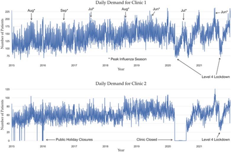
Figure 1. Daily patient demand at both urgent care clinic (UCC) clinics ranging from 2015 to 2021.
The annual patient volumes were aggregated by week across the entire longitudinal timeline and are illustrated in Figure 2. The resulting graphical plots demonstrate distinct drops in clinical demand during school vacation intervals, with prominent surges occurring during the mid-year influenza season and throughout the Christmas and New Year holiday period, when local general practice clinics are typically closed.
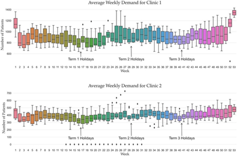
Figure 2. Average patient demand across both urgent care clinics (UCCs) for all years by week number.
Conversely, Figure 3 outlines the mean patient demand for both centers aggregated by the specific day of the week. A uniform trend across both locations is a distinct surge in clinical demand during weekend intervals when standard general practitioners do not operate, followed by a monotonic decline that reaches its lowest volume mid-week.
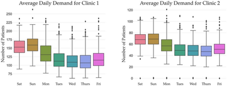
Figure 3. Average daily patient demand by day of the week across both urgent care clinics (UCCs).
The empirical data illustrated in Figures 1, 2, and 3 demonstrate powerful seasonal and cyclical weekly auto-correlation structures. To isolate these components and systematically determine the appropriate lagging thresholds for the predictor variables, we utilized auto-correlation function (ACF) plots, which measure the statistical relationship between current clinical demand and historical values. Figure 4 displays the daily, weekly, and monthly ACF profiles for Clinic 1. Recurrent seasonal cycles are visible, revealing robust correlations between active patient counts and historical values from 7 to 14 days prior, as well as high correlations with corresponding operational periods 1–3 years in the past.
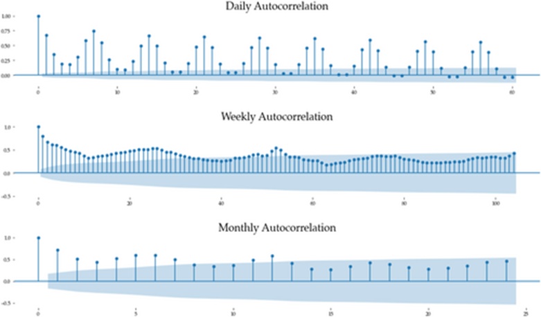
Figure 4. Auto-correlation plots (ACF) for Clinic 1.
Consequently, feature variables were engineered to represent historical lagging metrics from 7, 14, 364, 728, and 1092 days prior. The integration of a calendar variable capturing the week of the year accounted for the expanding baseline trend across the temporal timeline, as well as cyclical seasonal movements and school holiday schedules. A dedicated public holiday indicator binary flag ensured that the heightened patient volumes characteristic of these dates were explicitly represented within the feature space. To adjust for the impacts of COVID-19, an indicator variable was integrated to represent the legally mandated mobility restrictions implemented within the clinics' geographic region, mapping either the regional COVID-19 Alert Level architecture [23] or the subsequent Traffic Light regulatory frameworks [24] instituted by the New Zealand Government. Table 2 details the specific designations of all analytical variables used across the various figures alongside their comprehensive technical descriptions.
Table 2. Feature names as they appear in figures and their descriptions.
Feature | Explanation |
lag7d | Lagged value from 7 days earlier, representing the observation recorded one week before. |
lag14d | Lagged value from 14 days earlier, corresponding to the observation from two weeks before. |
lag1 | Lagged value from 364 days earlier, capturing the observation from one year prior. |
lag2 | Lagged value from 728 days earlier, representing the observation from two years prior. |
lag3 | Lagged value from 1092 days earlier, reflecting the observation from three years prior. |
public_holiday | Binary variable indicating whether the day is a public holiday (0/1). |
week | Calendar week index, taking values from 1 to 53. |
covid_level | COVID-19 restriction/alert level ranging from 1 to 4, or traffic-light status encoded as Green = 1 and Orange/Red = 2. |
To execute a mathematically rigorous validation of the candidate predictive frameworks, we constructed multiple benchmark configurations for comparative analysis. The initial baseline model replicates the historical internal methodology used by the clinical administrators to project prospective demand. This operational strategy involves applying a static 5% scaling increase to the historical patient aggregates recorded during the identical period of the preceding year. The secondary benchmark configuration, designated as the Naïve model, functions as a classical Random Walk framework [25], which operates under the assumption that the projected volume is mathematically identical to the observed volume from the corresponding period of the prior year. The tertiary baseline architecture was generated utilizing an ARIMA formulation [26]. Finally, an optimized variant of the Naïve architecture was engineered, which computes predictions for a specific day at a temporal point t by calculating the mean value of weighted historical lags across t-7, t-14, t-364, t-728, and t-1092 days.
We implemented eight distinct statistical and machine learning algorithms to produce competing predictive models. These configurations included Random Forest (RF) [27], Voting ensembles, Stacking architectures [28], Ridge Regression [29], and k-Nearest Neighbour Regression (kNN) [30] as executed via the Scikit-learn framework [31], alongside CatBoost [32], Prophet [33], and an Averaging Model. Table 3 presents a comprehensive summary of all evaluated algorithms and benchmark configurations, including their respective hyperparameter assignments where applicable. Beyond these baseline frameworks, we developed a mathematical mechanism to dynamically calibrate and refine the predictions generated by the Prophet and CatBoost models. We formulated two distinct modeling strategies to evaluate the historical residuals, utilizing these auxiliary models as adaptive correctives through the application of exponential smoothing and autoregressive formulations. The execution of both correction techniques across the two primary algorithms introduced four supplemental models to the total predictive matrix under evaluation.
Table 3. Summary of the benchmark models and algorithms used in this study, together with hyperparameter settings where applicable.
Approach | Summary |
Internal Forecasting Method | The forecasting procedure currently employed by the clinics assumes that patient demand on a specific day will be 5% greater than demand observed on the corresponding day of the preceding year. |
Naïve Forecasting Model | A baseline approach based on the random-walk concept [25], where the predicted value is simply taken as the observation from the equivalent period in the previous year. |
Improved Naïve Model | An enhanced benchmark technique that computes forecasts using a weighted average of historical observations at time lags t−7, t−14, t−364, t−728, and t−1092. The empirically optimized weights assigned to these lagged features were [2, 19, 26, 34, 35], with more recent observations receiving higher importance. |
ARIMA [26] | A classical autoregressive forecasting framework that estimates future observations by exploiting patterns contained in historical values. |
Ridge Regression [29] | A regression method that extends ordinary least squares by incorporating L2 regularization, shrinking coefficients toward zero to obtain a more parsimonious model and typically reducing variance and mean-squared error. |
kNN Regression [30] | A non-parametric prediction technique that relies on similarity between observations. Forecasts are generated by aggregating the values of k neighboring data points that are most comparable to the target instance. |
Prophet [33] | An automatically configurable additive forecasting model capable of capturing nonlinear behavior through yearly, weekly, and daily seasonal patterns, while also incorporating holiday effects and adapting to trend disruptions. |
Random Forest [27] | An ensemble-learning method composed of multiple decision trees trained on random subsets of features. The aggregation of these uncorrelated trees generally yields stronger predictive performance than any individual tree. |
CatBoost [32] | A gradient-boosting ensemble algorithm that constructs successive decision trees, each aiming to reduce prediction loss. The overall ensemble size is controlled by specifying the maximum number of trees. |
Voting Regressor [31] | A meta-ensemble approach that first trains several base learners—specifically Prophet, CatBoost, and Random Forest in this study—and then combines their outputs through a weighted aggregation mechanism to generate the final prediction. |
Averaging Model | A customized ensemble strategy derived from the voting regressor. It integrates predictions from five regression models (ARIMA, kNN, Ridge Regression, Random Forest, and CatBoost) while excluding the highest and lowest forecast values before calculating the final average prediction. |
Stacking [28] | An ensemble meta-estimator that uses the outputs of base models (Prophet, CatBoost, and Random Forest) as inputs to a higher-level regressor, whose prediction serves as the final forecast. |
The majority of machine learning algorithms incorporate numerous hyperparameters that can be assigned a wide spectrum of numerical values. It cannot be determined a priori which unique parametric configuration will generate the highest predictive accuracy across differing datasets. Consequently, standard data science practices dictate the use of methodologies that exhaustively or stochastically select hyperparameter values from a predefined grid or range, followed by the training and validation of multiple model permutations to isolate the optimal hyperparameter combination.
To isolate the appropriate hyperparameters for the algorithms evaluated in this study, we employed a grid search methodology that systematically evaluated an array of manually established parametric values. Hyperparameters do not exert uniform mathematical influence across all algorithmic structures regarding their impact on final model behavior. Table 4 highlights the specific hyperparameters targeted for optimization across each algorithm, alongside their predefined analytical ranges. Except where explicitly noted, standard default configurations were maintained for all unlisted hyperparameter values.
Table 4. Hyperparameter values for each algorithm used in the grid search optimisation approach.
Method | Description |
kNN | The k-nearest neighbors model was configured with k = 5, uniform weighting, and the Minkowski distance metric. |
ARIMA | An automatic ARIMA parameter optimization procedure was employed to determine the most suitable model configuration. |
CatBoost | Hyperparameter tuning explored max_depth = [4, 6, 8], learning_rate = [0.05, 0.1, 0.2], and ensemble_size = [100, 500, 1000]. |
Random forest | The random forest algorithm was evaluated using max_depth = [5, 10, 14, 18] and ensemble_size = [100, 500]. |
Prophet | Model calibration involved testing changepoint_prior_scale = [0.01, 0.05, 0.1]. |
Voting | Different weighting combinations for the constituent base models were examined, including [1,1,1], [1,2,3], [2,1,3], and [3,2,1]. |
Hyperparameter optimization was executed prior to validating the predictive frameworks against each respective test partition. The optimal hyperparameters were isolated from the training partition utilizing a standard k-fold cross-validation methodology.
The predictive frameworks were validated using longitudinal data spanning a three-year period from 2017 onward, utilizing an expanding window testing paradigm. The models were sequentially initialized and trained on historical data from 2014 to 2016, with forward projections computed starting 1 January 2017 up to 13 weeks (91 days) in advance. Figure 5 structurally details this validation architecture.
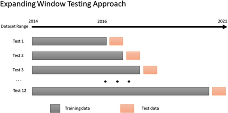
Figure 5. The expanding window testing approach used in this study. Each testing window represents 13 weeks, equivalent to 91-days ahead or one quarter.
When computing projections across each quarterly horizon, the generated forecast values iteratively became the input variables for subsequent downstream predictions. This recursive dependency specifically affected the 7-day and 14-day lagged variables; following the first and second week of the active forecast horizon, respectively, these parameters no longer had access to empirical observations within the dataset. Instead, they were systematically substituted with previously calculated model forecasts to precisely replicate the real-world operational challenges of long-range forecasting.
Upon completing the predictions for a given quarter, the training dataset window was expanded to incorporate the empirical observations from that newly completed period. The 91-day forecasting window was then advanced to predict the daily patient volume for the subsequent quarter. By systematically repeating this predictive cycle through the conclusion of 2019, we generated 12 distinct forecasting blocks, each encompassing daily predictions across a 91-day prospective horizon.
Projections were not calculated for the 2020 dataset due to the severe systemic disruptions caused by the pandemic and associated stay-at-home mandates, which resulted in compulsory, prolonged closures of certain clinical sites. However, the data from 2020 was preserved to train the machine learning frameworks, allowing them to model the structural shifts generated by the pandemic to predict 2021 volumes. Because of these COVID-19-induced structural anomalies, we isolate and examine the resulting model projections into two distinct categories: the years 2017–2019, representing stable, baseline historical demand patterns, and the year 2021, representing the volatile, pandemic-disrupted era.
To evaluate the predictive performance of the engineered frameworks, several mathematical validation metrics were deployed, each providing a distinct analytical viewpoint. These metrics were computed independently across both the 2017–2019 baseline timeline and the 2021 pandemic-disrupted dataset.
We report the Mean Absolute Percentage Error (MAPE) for each candidate algorithm. The mathematical formulation of MAPE is defined as:
 (1)
where T represents the total number of forecasted temporal horizons under evaluation, and et signifies the error or residual value computed from the mathematical difference between the empirically observed value yt and the corresponding model projection y at a specific point in time t. MAPE serves as an informative indicator because it expresses the deviations between observed parameters and model outputs as normalized percentages, making it intuitive to interpret. This metric is widely implemented within predictive literature and is academically endorsed as a primary benchmark for time-series evaluations [34]. Because it is scale-independent, MAPE enables the direct comparison of model performance across disparate datasets characterized by completely different baseline scales—such as the distinct patient volume magnitudes recorded between Clinic 1 and Clinic 2—while also allowing cross-study evaluations against external published research.
Additionally, the Root Mean Square Error (RMSE) was adopted as our primary error variance metric, formulated as follows:
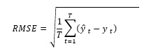 (2)
The RMSE provides valuable operational insight by detailing the variance and distribution of the residuals while retaining the same units as the dependent variable; lower numeric outputs indicate superior model alignment.
To comprehensively aggregate the mathematical performance of all candidate algorithms across the complete matrix of validation partitions, a mean ranking methodology was executed. For every separate 91-day forecasting block, each of the twelve algorithms was assigned a ordinal rank from 1 to 12 based on its calculated MAPE score, with a rank of one denoting the most accurate model configuration. This step was performed systematically across all 12 testing blocks to compute the final mean rank for each framework.
For analytical completeness, we additionally report the Mean Absolute Error (MAE) across all models, which mirrors the validation framework established by Zhang et al. [9]. The MAE represents the average absolute geometric deviation between the observed data points and the projected outcomes. Consequently, it is conceptually straightforward to evaluate and remains less sensitive to outlier anomalies than RMSE, which penalizes larger deviations more heavily through quadratic squaring. Thus, a small number of substantial forecasting errors will affect the final RMSE calculation to a significantly greater degree than the MAE. The mathematical calculation for MAE is structured as:
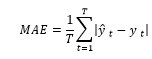 (3)
While the descriptive metrics detailed above are sufficient to identify disparities in absolute predictive precision among the models, they cannot determine whether the underlying forecast distributions differ at a level of true statistical significance. To establish this, we applied the Diebold–Mariano [36] statistical test, executing pairwise comparisons to verify whether the sequences of model residuals were meaningfully distinct from one another. We formally compared the output vectors of each candidate machine learning model against the baseline in-house scheduling methods, while also conducting cross-examinations between the top-performing algorithmic architectures.
The substantial increases in predictive capability and architectural complexity found in contemporary machine learning algorithms are inherently accompanied by a corresponding deficit in the conceptual interpretability of the resulting frameworks, alongside a reduced capacity to provide explanations for their outputs. This transparency deficit has emerged as a major concern due to escalating regulatory frameworks and public policy mandates demanding greater structural visibility within automated predictive modeling [37].
The mandate to resolve this operational challenge has driven the development of the emerging discipline of XAI. A robust array of diagnostic instruments has recently been engineered to address this issue, attempting to systematically explain the underlying logic behind machine learning predictions. Two methodologies are currently recognized as the state of the art within the XAI domain [38]: namely, Local Interpretable Model-agnostic Explanations (LIME) [39] and SHapley Additive exPlanations (SHAP) [40]. Both frameworks are deployed in tandem throughout this study.
We leverage these analytical tools to scrutinize the behavioral mechanics of our predictive frameworks at both global and local operational scales. At a global resolution, our focus centers on isolating the aggregate mathematical influence that each unique feature exerts across the model's entire output space. To achieve this, we utilize feature importance plots that visually rank and illustrate the relative weights of each variable. We also evaluate feature importance visualizations that map the functional changes in final forecasts caused by shifting individual input values. Together, these graphical tools offer high-level interpretability regarding the primary drivers of a given model. Conversely, when evaluating model mechanics at a local resolution, we seek to extract an explicit explanation from the framework regarding the exact mathematical reasons it generated a specific forecast for a single, isolated data point.
Both the SHAP and LIME frameworks operate by constructing secondary models that mathematically approximate the localized predictions and behavioral profiles of the underlying "black-box" systems. These auxiliary frameworks are defined as surrogate models and are explicitly configured to maximize human interpretability. Because these surrogate structures are trained to precisely mimic the internal dynamics of the primary machine learning algorithms, researchers can extract valid insights concerning the actual models by interpreting these accessible surrogates. The surrogate systems learn to replicate the primary model's behavior by systematically perturbing the underlying input vectors—mirroring traditional sensitivity analysis—and subsequently recording the variations within the final model output space. Through this mechanism, the surrogates map changes in model projections driven by incremental adjustments to the input variables. This operational principle allows us to calculate the true magnitude and importance of specific data features: if a minor perturbation in a given variable triggers a substantial change in the final forecast vector, it can be mathematically deduced that the variable represents a critical predictor within the model.
The SHAP framework relies fundamentally on the calculation of Shapley values [41], which adapt cooperative game theory principles to allocate each individual feature's marginal economic contribution to the final predictive outcome in combination with all other concurrent variables. Consequently, SHAP is capable of generating mathematically unified explanations across both global and local resolutions.
In contrast, LIME operates exclusively at a localized scale. It constructs an inherently interpretable model—selected from classical candidate algorithms such as Linear Regression, Lasso, or Decision Trees—by utilizing weighted, simulated data samples drawn from the immediate geographic proximity of the specific target observation for which an explanation is required.
These diagnostic frameworks are not without mathematical limitations. Despite the rigorous theoretical foundation of SHAP, the computational complexity of calculating exact Shapley values scales exponentially relative to the number of integrated features, rendering precise computation intractable as the feature space expands; thus, heuristic approximation algorithms must be deployed. An additional limitation of SHAP is its tendency to occasionally generate highly unrealistic synthetic input vectors when training the surrogate model, which can compromise the integrity of the resulting insights. On the other hand, LIME requires an empirical trial-and-error configuration process spanning a wide range of tunable hyperparameters to construct a logical surrogate model. Furthermore, LIME can suffer from localized instability, meaning that explanations generated for two highly proximal data points may diverge significantly from one another [35]. For these reasons, and because of the differing analytical perspectives offered by each approach, it is mathematically more robust to deploy both techniques in tandem when examining the interpretability of a predictive framework.
Table 5 details the mean RMSE, MAE, and MAPE metrics alongside the combined mean rankings calculated across the 12 distinct prospective horizons generated between 2017 and 2019 for each candidate framework. The top four performing models, isolated by the lowest (i.e., most optimal) mean ranks relative to their MAPE outputs, are highlighted in bold. For Clinic 1, the superior architectures were the Voting ensemble, the Averaging model, the Stacking configuration, and the Prophet framework. An identical performance pattern emerged for Clinic 2, where the Stacking architecture yielded the lowest absolute error rates. The empirical results demonstrate that the error-correction mechanisms designed to calibrate model outputs via autoregressive and exponential smoothing formulations successfully generated superior precision compared to the baseline benchmarks; however, they were unable to outperform the top-tier ensemble configurations. Every proposed machine learning architecture demonstrated a clear performance improvement over the historical in-house forecasting techniques and the majority of standard baseline models across the 2017–2019 dataset. A visualization of the operational forecasting behavior of the Voting ensemble utilizing Clinic 1 data across all four quarters of 2019 is illustrated in Figure 6, plotted directly against the empirically observed patient flows.
Table 5. Model forecast accuracies on 2017–2019 data. [R] denoting mean ranks, [*] mean ranking per clinic, and [+] the combined mean ranking over both clinics, which is used to order all the results—the best performing algorithms appearing at the bottom and are in bold.
Model | Combined clinics | Clinic 2 |
|
|
| Clinic 1 |
|
| |
R+ | R* | MAPE | MAE | RMSE | R* | MAPE | MAE | RMSE | |
Naïve | 13.6 | 13.2 | 17.2 | 11.1 | 13.8 | 14.0 | 12.7 | 18.5 | 22.9 |
Current in-house approach | 13.3 | 12.8 | 17.4 | 10.9 | 13.6 | 13.7 | 12.4 | 17.7 | 21.9 |
ARIMA | 11.0 | 10.3 | 16.5 | 9.7 | 11.8 | 11.6 | 14.0 | 20.0 | 23.8 |
CatBoost + Exponential Smoothing | 10.2 | 10.8 | 15.9 | 9.9 | 12.5 | 9.5 | 10.9 | 15.4 | 19.2 |
Prophet + Exponential Smoothing | 9.9 | 12.0 | 16.1 | 9.8 | 12.2 | 7.8 | 10.9 | 15.5 | 19.0 |
kNN | 9.3 | 8.4 | 14.1 | 9.2 | 11.5 | 10.2 | 10.5 | 15.3 | 19.3 |
Enhanced Naïve model | 9.0 | 6.8 | 14.1 | 9.3 | 11.4 | 11.2 | 11.2 | 16.6 | 20.4 |
CatBoost + Autoregression | 9.0 | 9.6 | 15.2 | 9.4 | 11.9 | 8.3 | 10.2 | 14.5 | 18.1 |
CatBoost | 8.7 | 8.6 | 14.3 | 9.3 | 11.8 | 8.7 | 9.9 | 14.4 | 18.0 |
Prophet + Autoregression | 8.1 | 10.1 | 15.4 | 9.4 | 11.9 | 6.0 | 10.2 | 14.6 | 17.8 |
Random Forest | 7.7 | 7.9 | 14.1 | 9.1 | 11.7 | 7.5 | 9.6 | 13.9 | 17.6 |
Ridge Regression | 7.6 | 7.3 | 13.7 | 8.8 | 11.4 | 7.9 | 9.5 | 13.9 | 17.3 |
Prophet | 5.3 | 5.6 | 13.2 | 8.2 | 10.9 | 5.0 | 9.3 | 13.3 | 16.4 |
Averaging Ensemble | 4.7 | 4.0 | 12.8 | 8.2 | 10.6 | 5.4 | 9.0 | 12.9 | 16.0 |
Stacking Ensemble | 4.6 | 4.3 | 12.8 | 8.0 | 10.3 | 4.8 | 9.1 | 13.1 | 16.2 |
Voting Ensemble | 4.5 | 4.4 | 12.8 | 8.2 | 10.6 | 4.6 | 8.9 | 12.8 | 15.9 |
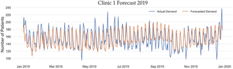
Figure 6. Example forecast plot for 2019 showing actuals versus forecasted values for Clinic 1 by the voting model.
Although the empirical data in Table 5 establishes that the proposed machine learning frameworks operate with higher precision than the baseline models across multiple dimensions, we conducted supplemental statistical tests to verify if the outputs of the top-performing algorithms were truly distinct from the traditional in-house scheduling strategies at an acceptable level of statistical significance. Relying on the Diebold–Mariano validation test, the mathematical outputs confirmed that the 12 forecast sequences generated between 2017 and 2019 by each proposed model were significantly different (at the 0.01 significance level) from the clinical in-house estimations.
Furthermore, we executed pairwise Diebold–Mariano examinations across the forecast vectors of the top-performing algorithms. For the Clinic 1 projections, the vast majority of model pairings demonstrated statistically significant differences (at the 0.05 level) from one another, with the exception of the Stacking, Averaging, and Prophet configurations. For Clinic 2, nearly all model pairings could be classified as significantly different from one another, except for the comparisons of CatBoost versus Random Forest, Voting versus Prophet, and the Averaging framework versus the Stacking, Voting, and Prophet models.
We now evaluate the predictive characteristics of the proposed frameworks across the 2021 dataset, which captures the turbulent, unstable operational patterns induced by pandemic-era healthcare conditions. We initially observe the aggregated performance of the models across this timeline using multiple evaluation metrics, as structured in Table 6. The resulting metrics reinforce that, across both clinical sites, the Voting ensemble generated the highest degree of generalizability on average according to the MAPE index, while the Prophet framework and the Averaging model achieved the second and third positions, respectively. Regarding the discrepancy in model accuracy between the two facilities, the calculated MAPE scores indicate that producing precise long-range forecasts for 2021 was substantially more difficult for Clinic 2 than for Clinic 1. The MAPE metrics demonstrate that the absolute errors recorded for Clinic 2 were roughly 50% higher than those calculated for Clinic 1. We can infer from this statistical variance that Clinic 2 experienced a higher susceptibility to pandemic-induced operational disruptions than Clinic 1, an assertion supported by the heightened volatility visible within the empirical raw data in Figure 1.
Table 6. Model forecast accuracies for 2021. [R] denoting mean ranks, [*] mean ranking per clinic, and [+] the mean ranking over both clinics, which is used to order all the results – the best-performing algorithms appearing at the bottom and are in bold.
Model | Combined clinics | Clinic 2 |
|
|
| Clinic 1 |
|
| |
R+ | R* | MAPE | MAE | RMSE | R* | MAPE | MAE | RMSE | |
Naïve | 13.6 | 13.2 | 17.2 | 11.1 | 13.8 | 14.0 | 12.7 | 18.5 | 22.9 |
Current in-house approach | 13.3 | 12.8 | 17.4 | 10.9 | 13.6 | 13.7 | 12.4 | 17.7 | 21.9 |
ARIMA | 11.0 | 10.3 | 16.5 | 9.7 | 11.8 | 11.6 | 14.0 | 20.0 | 23.8 |
CatBoost + Exponential Smoothing | 10.2 | 10.8 | 15.9 | 9.9 | 12.5 | 9.5 | 10.9 | 15.4 | 19.2 |
Prophet + Exponential Smoothing | 9.9 | 12.0 | 16.1 | 9.8 | 12.2 | 7.8 | 10.9 | 15.5 | 19.0 |
kNN | 9.3 | 8.4 | 14.1 | 9.2 | 11.5 | 10.2 | 10.5 | 15.3 | 19.3 |
Enhanced Naïve model | 9.0 | 6.8 | 14.1 | 9.3 | 11.4 | 11.2 | 11.2 | 16.6 | 20.4 |
CatBoost + Autoregression | 9.0 | 9.6 | 15.2 | 9.4 | 11.9 | 8.3 | 10.2 | 14.5 | 18.1 |
CatBoost | 8.7 | 8.6 | 14.3 | 9.3 | 11.8 | 8.7 | 9.9 | 14.4 | 18.0 |
Prophet + Autoregression | 8.1 | 10.1 | 15.4 | 9.4 | 11.9 | 6.0 | 10.2 | 14.6 | 17.8 |
Random Forest | 7.7 | 7.9 | 14.1 | 9.1 | 11.7 | 7.5 | 9.6 | 13.9 | 17.6 |
Ridge Regression | 7.6 | 7.3 | 13.7 | 8.8 | 11.4 | 7.9 | 9.5 | 13.9 | 17.3 |
Prophet | 5.3 | 5.6 | 13.2 | 8.2 | 10.9 | 5.0 | 9.3 | 13.3 | 16.4 |
Averaging Ensemble | 4.7 | 4.0 | 12.8 | 8.2 | 10.6 | 5.4 | 9.0 | 12.9 | 16.0 |
Stacking Ensemble | 4.6 | 4.3 | 12.8 | 8.0 | 10.3 | 4.8 | 9.1 | 13.1 | 16.2 |
Voting Ensemble | 4.5 | 4.4 | 12.8 | 8.2 | 10.6 | 4.6 | 8.9 | 12.8 | 15.9 |
The individual quarterly projections for 2021 are broken down by MAPE in Table 7. As shown in the data, predicting fourth-quarter trends proved highly problematic for both facilities, while the third quarter presented unique forecasting difficulties specifically for Clinic 2. To better understand these dynamics, Figure 7 illustrates the actual versus predicted outputs generated by the Voting model for Clinic 1 across the entirety of 2021. The visualization highlights a stark divergence between the model's predictions and actual observations during the final quarter. It is important to emphasize that because these models operate on a one-quarter-ahead predictive framework, they cannot account for subsequent, unexpected shifts in the clinical operating environment. For instance, the fourth-quarter projections for Clinic 1 were generated during the preceding quarter, right as the initial SARS-CoV-2 Delta variant outbreak emerged in the Auckland region. Following this outbreak, local general practitioners made an unprecedented, widespread shift to halt in-person visits and move entirely to virtual care. This primary care shutdown persisted well into the fourth quarter—even as official COVID-19 Alert Levels began to ease—causing a massive, compounding spike in patient volume at the UCC. This scenario underscores the fundamental challenge of managing extended forecasting horizons during highly volatile, unprecedented disruptions.
Table 7. Model metrics forecasting 2021. [R] denoting mean ranks, [*] mean ranking per clinic, and [+] the mean ranking over both clinics, which is used to order all the results – the best-performing algorithms appearing at the bottom and are in bold.
Model | Combined Clinics | Clinic 2 |
|
|
|
| Clinic 1 |
|
|
| |
R+ | R* | Q4 | Q3 | Q2 | Q1 | R* | Q4 | Q3 | Q2 | Q1 | |
CatBoost | 4.5 | 3.8 | 30.0 | 22.4 | 11.9 | 18.1 | 5.3 | 27.9 | 13.5 | 10.2 | 12.3 |
Random Forest | 4.4 | 4.5 | 27.6 | 38.5 | 12.3 | 18.6 | 4.3 | 25.8 | 11.4 | 9.2 | 13.0 |
Stacking Ensemble | 4.1 | 3.5 | 31.0 | 20.3 | 12.8 | 16.5 | 4.8 | 26.1 | 12.6 | 12.2 | 12.1 |
Averaging Ensemble | 3.1 | 3.3 | 27.1 | 21.1 | 12.9 | 16.4 | 3.0 | 23.1 | 10.7 | 10.4 | 10.8 |
Prophet | 2.9 | 3.3 | 22.1 | 28.2 | 17.7 | 15.7 | 2.5 | 17.1 | 11.7 | 9.8 | 9.7 |
Voting Ensemble | 2.0 | 2.8 | 23.7 | 20.4 | 13.8 | 15.8 | 1.3 | 21.9 | 10.2 | 8.8 | 10.0 |
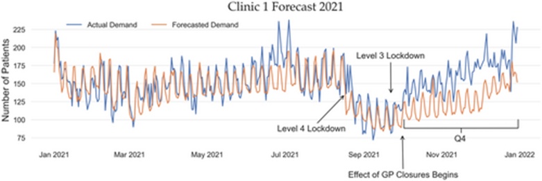
Figure 7. Example forecast plot for 2021 showing actuals versus forecasted values for Clinic 1.
The overall accuracy of the top proposed models is detailed in Table 8, measured by their mean percentage improvement over historical in-house estimation baselines. The results demonstrate that the Voting ensemble was consistently the most effective framework for both locations. Specifically for Clinic 1, the Voting model boosted accuracy by 28% for the 2017–2019 baseline data and by 16% during the 2021 period. For Clinic 2, performance gains over the traditional in-house approaches ranged from a 25% improvement for the 2017–2019 dataset to a 30% improvement for the 2021 dataset.
Table 8. Model improvements over the current in-house benchmark model for data ranging 2017–2019 and 2021.
Clinic 2 |
| Clinic 1 | ||
Model | 2021 | 2017–2019 | 2021 | 2017–2019 |
CatBoost | 21% | 16% | −5% | 19% |
Random forest | 15% | 18% | 3% | 22% |
Stacking | 21% | 24% | −3% | 26% |
Prophet | 23% | 21% | 23% | 24% |
Averaging | 26% | 25% | 9% | 27% |
Voting | 30% | 25% | 16% | 28% |
The preceding analysis highlights the inherent friction encountered when generating long-range predictions. To visualize this, Figure 8 tracks the collective variance in forecast errors for the Voting model across a standard 91-day predictive window. This graph charts the average residual error relative to the number of days advanced across the full spectrum of model-generated forecasts. The data reveals that the error margins remain remarkably stable throughout the majority of the 91-day horizon. Expectedly, predictability and error control are strongest during the initial weeks, as these early forecasts directly leverage actual 7- and 14-day lag inputs. Conversely, a noticeable rise in error variance occurs around day 85, marking the specific threshold where predictive accuracy begins to degrade.
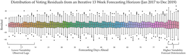
Figure 8. Forecast stability as an aggregate across all the 13-week forecast horizons for Clinic 1.
To evaluate the internal mechanics and predictive logic of the Voting model, we utilize SHAP and LIME interpretability frameworks. Furthermore, we break down individual feature importance metrics for the standalone CatBoost and Random Forest models, given that the final Voting ensemble aggregates these two architectures alongside the Prophet model.
To evaluate model behavior across contrasting conditions, we analyze several distinct forecasting windows. We examine the Voting model's performance during Q2 2018 and Q4 2019 to establish a baseline for normal, stable data environments. These predictable periods are then contrasted against Q1 2021, a highly volatile window defined by pandemic-induced lockdowns. Additionally, we isolate how the model handles non-standard, high-impact events like public holidays, which typically trigger dramatic shifts in patient volume. For this analysis, we evaluate model explainability regarding Easter and school holiday patient distributions while measuring the specific weight of individual features.
The predictive outputs for Q2 2018 are visualized in Figure 9, which provides a global-level diagnostic analysis of the model's internal logic from multiple angles.
Figures 9a and 9b present the internal feature rankings calculated natively by CatBoost and Random Forest. These plots order the attributes by their predictive weight and illustrate the relative scale of each feature's impact. In parallel, Figure 9c displays both the overall feature importance and the directional shift in predictions caused by varying feature inputs. Crucially, the diagnostics in Figure 9c are derived via a SHAP surrogate model. While each analysis framework offers a distinct mathematical lens, evaluating them collectively allows for a reliable triangulation of data, ensuring a more robust empirical foundation for our findings.
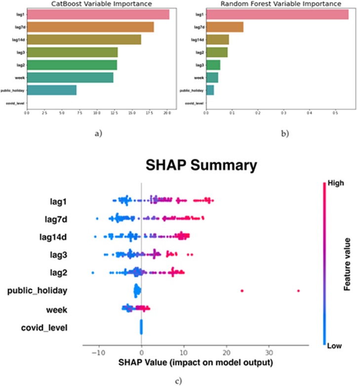
Figure 9. Variable importance plots Q2 2018 showing outputs from (a) CatBoost, (b) Random Forest (RF) and (c) SHAP.
All three analytical lenses consistently identify the primary drivers of patient demand during this timeframe as historical lookbacks: specifically, data matching the same calendar day from 1 year, 1 week, and 2 weeks prior. This indicates that under baseline operating conditions, long-term historical patterns (the previous year's data) exert a stronger influence on the model's predictions than immediate recency (1- to 2-week lags). Notably, the Random Forest architecture heavily prioritizes the 1-year lag variable compared to CatBoost, which aligns more closely with the SHAP rankings. Extended lookbacks from 2 and 3 years prior emerge as the secondary tier of influential features, though their exact order fluctuates slightly depending on the diagnostic tool used. Calendar attributes, such as the week of the year and public holiday indicators, are ranked next by CatBoost and Random Forest, whereas SHAP places these two in reverse order. As expected for a pre-pandemic dataset, all models treat the COVID-19 Alert Level feature as entirely non-influential.
The SHAP summary visualization in Figure 9c introduces an extra layer of global interpretability by illustrating how upward or downward shifts in a feature's value mathematically alter the final prediction. In this plot, color coding signifies input values (red for high, blue for low), while the horizontal axis charts the resulting SHAP values. Data points plotted to the right of the vertical zero axis indicate a positive predictive push, meaning those values drive the model to forecast higher patient volumes. Conversely, data points on the left indicate a negative impact, lowering the projected demand. The distance a point travels from the center line directly correlates to its overall influence on the final output.
Based on Figure 9c, elevated values for the top two historical features trigger a disproportionately stronger response in the final forecast compared to lower values. Put simply, the model scales up its patient volume projections intensely if the previous year or week showed high traffic, but it reacts with less intensity when those same markers are low. This demonstrates a clear upward directional bias for these primary features. In contrast, the next three variables—the 14-day, 3-year, and 2-year lags—exhibit a more symmetric, balanced effect on the outputs. The public holiday feature functions as a binary switch; standard non-holiday days prompt a mild downward adjustment in projected demand. However, the distinct data points capturing actual public holidays (such as Easter Monday, Queen's Birthday, and ANZAC Day) demonstrate just how aggressively the model spikes its volume projections for these specific dates. Finally, the week number typically applies a downward pull on the forecast. Yet, as the second quarter moves forward into late autumn and approaches both winter and the peak influenza season, the week number variable shifts behavior, driving the final patient demand projections upward.
To verify the consistency and reproducibility of this explainability framework, we replicated the interpretability analysis on the Q4 2019 forecasting window—representing the final baseline period preceding the pandemic, as illustrated in Figure 10. Selecting an alternate non-disrupted timeframe confirms that the underlying model mechanics reliably mirror the behaviors observed during the Q2 2018 window.
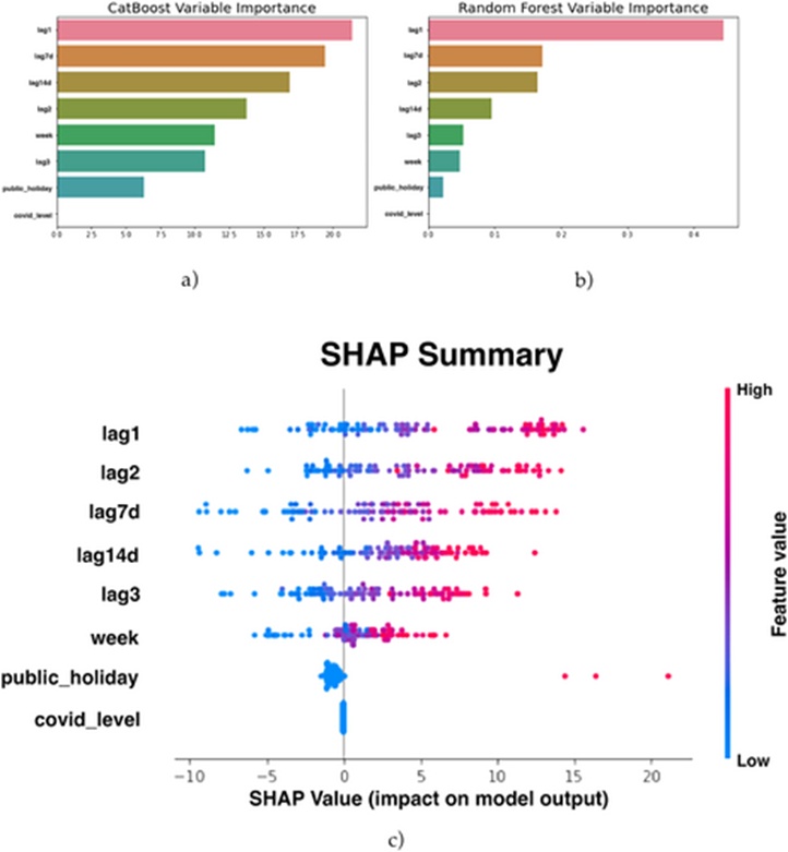
Figure 10. Variable importance plots for Q4 2019 showing outputs from (a) CatBoost, (b) Random Forest (RF) and (c) SHAP.
Figures 10a and 10b confirm a strong alignment between both core models regarding feature weights, matching the trends seen in the Q2 2018 analysis. The SHAP outputs in Figure 10c, however, surface a few distinct nuances. Notably, historical data from 2 years prior takes on elevated importance during fourth-quarter forecasting. This shift aligns with seasonal expectations, as the fourth quarter regularly sees a progressive acceleration in patient volumes, culminating in a sharp peak every December. Because of this predictable annual ramp-up, long-term historical year-over-year markers become cleaner indicators for the model than immediate short-term fluctuations from the preceding weeks. Similarly, higher week numbers show an amplified effect on driving up demand projections as the year winds down. This matches our earlier seasonal observations, but becomes even more pronounced in the final quarter due to the traditional closure of local general practices over the extended summer holiday break. Furthermore, the graphics reinforce the heavy mathematical weight assigned to public holidays; the three specific holidays falling within this quarter (Labour Day, Christmas Day, and Boxing Day) serve as powerful drivers that drastically elevate the model's patient volume forecasts for those dates.
This high level of behavioral uniformity between the Q4 2019 and Q2 2018 windows is highly indicative of the feature dynamics observed across all stable, pre-pandemic horizons (2017–2019). Consequently, it is evident that under normal clinical operations, the foundational driver of a forecast is the same-day demand from the prior year, which anchors the model's baseline stability. This is balanced by the 7- and 14-day lag inputs, which inject essential responsiveness, allowing the model to adapt to fast-moving, real-time healthcare shifts—such as seasonal flu outbreaks or sudden respiratory surges that introduce an unpredicted, stochastic element to clinical demand.
To evaluate how models perform under disruptive conditions, predictions from the pre-pandemic era can be compared against a representative window from Q1 2021, where the underlying data matrix was heavily distorted by COVID-19 anomalies (Figure 1). Consequently, this specific forecasting window serves as an ideal baseline for evaluating how different variables contribute to model flexibility and real-time adjustment during non-standard operational periods. The internal logic of these models during this timeframe is illustrated in Figure 11.
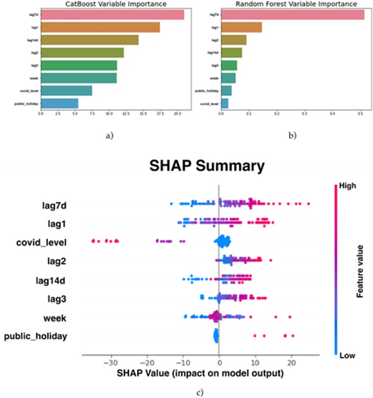
Figure 11. Variable importance plots for Q1 2021 showing outputs from (a) CatBoost, (b) Random Forest (RF) and (c) SHAP.
The analytical outputs show strong structural alignment between the internal rankings of CatBoost (Figure 11a) and Random Forest (Figure 11b), with both models reaching a consensus with the SHAP framework (Figure 11c) regarding the two primary variables. Under these unstable conditions, immediate short-term data—specifically the 7-day historical lag—supersedes the highly anomalous, pandemic-skewed 1-year lookback data from 2020 as the primary driver of the system's predictions. This represents a complete inversion of pre-pandemic behaviors, where the 1-year historical baseline served as the anchor for the system, reflecting an implicit structural assumption of long-term operational stability. Furthermore, the SHAP diagnostics demonstrate that the active COVID-19 Alert Level emerged as a statistically significant contributor to the finalized outputs, a dynamic that was entirely absent during non-pandemic baseline periods. As shown in the SHAP overview, elevated alert levels correlate with a sharp downward adjustment in predicted patient volume, whereas low alert values exert almost no influence. This mathematical behavior aligns with real-world observations, given that periods under Alert Level 4 triggered a substantial contraction in overall clinical presentations compared to standard operational windows under Alert Level 1.
At this stage, the analytical focus shifts from an aggregate, macro-level diagnostic to a localized, instance-specific evaluation of model behavior. Retaining the Q1 2021 evaluation window, this section isolates the precise mathematical impacts that shifting COVID-19 Alert Levels exert on localized predictions. By leveraging explainable artificial intelligence (XAI) frameworks, we expose the underlying computational logic driving individual data points. Specifically, we audit model performance across two distinct dates defined by contrasting policy environments: one representing an active Alert Level 1 status, and the other occurring under Alert Level 3 restrictions. These localized dynamics are captured across Figures 12 and 13.
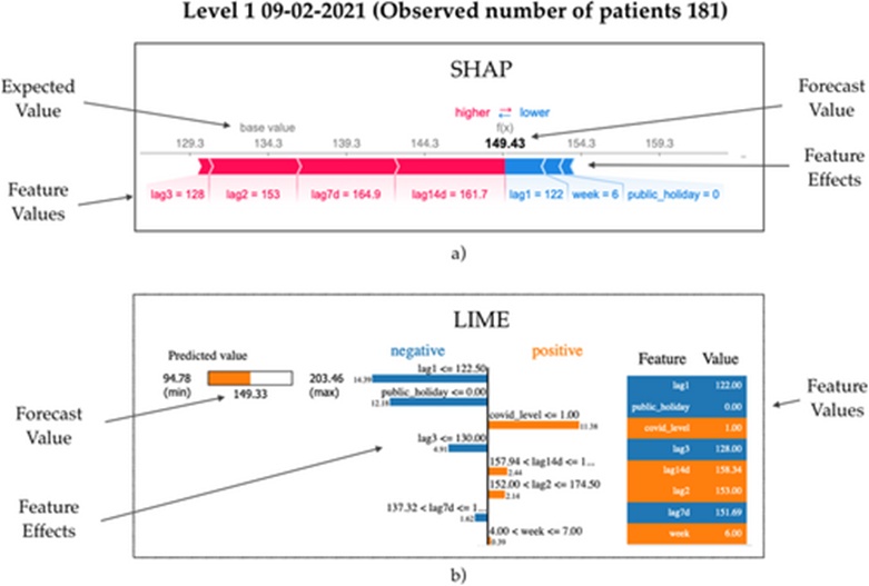
Figure 12. Model explainability showing the reasoning behind a forecast during COVID-19 Alert Level 1 2021 using (a) SHAP and (b) LIME.
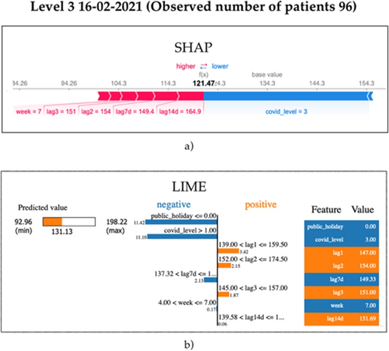
Figure 13. Model explainability showing the reasoning behind a forecast during COVID-19 Level 3 2021 using (a) SHAP and (b) LIME.
The instance-level behavior of the CatBoost model is mapped using the SHAP force framework in Figure 12a, while the corresponding Random Forest architecture is deconstructed via LIME in Figure 12b; both diagnostics target an Alert Level 1 scenario occurring on Tuesday, 9 February 2021. In Figure 12a, the baseline intercept (134 patients) denotes the expected mathematical mean across all historical observations, establishing a default prediction assuming unperturbed conditions. The finalized model output is highlighted in bold (149 patients projected versus an actual empirical count of 181). This visual mapping highlights how competing variables interact, with specific parameters driving the projection above the baseline mean (indicated by the red vectors) and opposing variables dragging the prediction downward (indicated by the blue vectors). This diagnostic shows that the 7-day and 14-day historical lags serve as the primary drivers pulling the prediction upward on this specific day, with vector length reflecting the underlying effect size. Conversely, the 1-year historical lag and the calendar week number exert minor downward pressure.
This behavior is validated by the LIME diagnostic in Figure 12b, which arrives at an identical total system projection of 149. The central pane charts the localized rule-based surrogate logic, illustrating the specific thresholds and mathematical coefficients optimized by LIME to emulate the internal operations of the underlying Random Forest model. The features are arranged sequentially based on their explanatory weight. The 1-year historical lookback and the fact that the target date fell on a standard business day (non-holiday status) function as the primary negative drivers, suppressing the forecast from its theoretical upper ceiling of 203 patients (left pane). Concurrently, the low active alert status (Level 1) acts as a positive counterbalance, preventing the projection from collapsing toward its theoretical lower limit of 95 patients.
Exactly one week later, the Auckland region escalated to COVID-19 Alert Level 3. Figure 13 captures the SHAP and LIME explanatory breakdowns for this high-restriction scenario, where the actual empirical count registered at 96 clinical arrivals. As shown in the SHAP force plot (Figure 13a), the dominant negative vector suppressing the total projection is the elevated alert level value. Conversely, the 7-day and 14-day historical lags (which carried over volume data from the preceding Alert Level 1 period) act as positive counterweights, pulling the projection upward to settle at a finalized output of 121 patients. This dynamic is reinforced by the LIME output in Figure 13b, where both the public holiday indicator and the active alert level function as the primary drivers of lower volume forecasts. However, in contrast to the SHAP framework, the LIME surrogate model indicates that the 1-year and 2-year historical lookbacks applied positive pressure toward higher volume expectations. Collectively, both diagnostic frameworks confirm that the models are highly sensitive to shifting alert level parameters, while providing transparency into how the remaining historical variables interact to calibrate output accuracy.
To isolate the explicit mathematical impact of the public holiday variable on system calibration, this section evaluates model behavior during a known calendar anomaly: Easter Monday (02-04-2018). The actual empirical demand recorded for this date was 154 patient presentations. From the SHAP diagnostic perspective detailed in Figure 14a, the model demonstrates a pronounced reaction to the active holiday indicator, which functions as the primary upward vector driving the finalized prediction toward 167. This dominant variable is supported by minor positive contributions from the 3-year and 7-day historical lags, while the remaining system features exert negligible downward pressure.
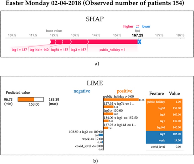
Figure 14. Model explainability showing the reasoning behind a forecast on Easter Monday 2018 using (a) SHAP and (b) LIME.
The corresponding instance-level prediction interpreted by the LIME framework in Figure 14b centers on an output value of 153, demonstrating exceptional proximity to the real-world observation. LIME’s behavioral diagnostic strongly aligns with the SHAP findings, confirming that flagging the target date as an active public holiday serves as the single most influential lever for scaling up the system's predictions. Similarly to the SHAP output, the 7-day short-term lag and the 3-year historical lookback provide auxiliary positive pressure. These combined results validate the functional utility of the public holiday parameter, demonstrating its capacity to accurately modulate predictions during severe calendar shifts and protect overall system reliability.
As a final diagnostic verification, we replicate this explainability approach to evaluate model mechanics on dates falling within standard school vacation blocks. Insights from domain experts indicate that school holiday intervals regularly depress typical patient volumes across both clinical facilities. Although initial efforts focused on engineering a dedicated, standalone feature to flag school holidays, empirical testing revealed that combinations of existing historical lag variables were structurally sufficient to convey this seasonal variance to the models. To illustrate this capacity, we audit model performance on a school holiday date: Friday 04-10-2019, with the corresponding explanatory logic mapped in Figure 15.
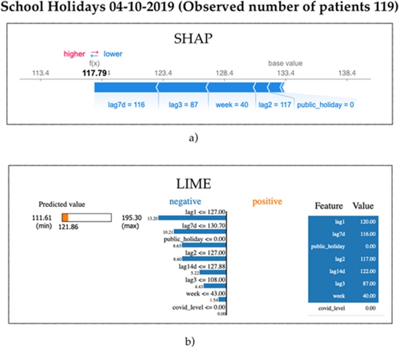
Figure 15. Model explainability showing the reasoning behind a forecast during school holidays in 2019 using (a) SHAP and (b) LIME.
The SHAP diagnostic output in Figure 15 establishes a baseline intercept value of 133 patients against an actual recorded volume of 119 arrivals. The visualization demonstrates that the required downward correction is driven by a cooperative interaction of features: specifically, the 7-day lag, the 3-year lag, and the calendar week number, which collectively suppress the final system output to 118 patients.
An identical operational dynamic is surfaced by the LIME surrogate model, where the 1-year, 2-year, and 7-day historical lookbacks—evaluated alongside the binary public holiday indicator—operate in tandem to drive the localized prediction downward to 122 patients. These findings indicate that historical lag metrics, when evaluated in combination with temporal features, naturally internalize the seasonal disruptions caused by school vacation periods. Consequently, the ensemble models retain sufficient information to autonomously depress patient volume forecasts during these intervals, eliminating the need to construct extra, hyper-specific variables that could increase the risk of overparameterization and model overfitting.
In response to RQ1, our findings firmly establish that machine learning architectures can be successfully deployed to project patient demand at UCCs, offering substantial performance gains over existing in-house frameworks and standard benchmarks. Empirical evidence shows that during the pre-pandemic era, the predictive accuracy of the top-performing configurations yielded an improvement of 25% to 28% relative to baseline in-house strategies. Although the onset of the COVID-19 pandemic in New Zealand and its attendant operational restrictions introduced significant volatility that moderately elevated model error rates, the resulting projections maintained a clear advantage over both internal clinical methods and competing benchmark models. Throughout this disrupted interval, the proposed systems achieved accuracy improvements over in-house benchmarks ranging from 16% to 30% across both medical facilities.
Generating reliable projections across a 3-month predictive window is inherently challenging due to unobserved variables that manifest post-forecast and alter true healthcare utilization patterns. This phenomenon was clearly illustrated during Q4 2021, when a regional surge in SARS-CoV-2 Delta variant cases prompted the majority of local primary care offices to suspend in-person operations. This systemic contraction in primary care access subsequently triggered an abrupt escalation in patient volume at regional UCCs. Because long-term predictive models cannot capture such downstream, real-time systemic disruptions at their initialization point, these findings emphasize that, under stable conditions, the top-performing ensemble architectures maintain strong reliability even when approaching the maximum 91-day forecasting limit.
To evaluate these long-term predictive outputs within the broader academic landscape, the results must be contextualized alongside historical benchmarks documented in the literature (Table 1). Extant studies reporting on short-term, single-day-ahead projections typically describe error metrics ranging from 3% to 12% MAPE. Conversely, the sparse empirical evidence available for 30-day-ahead intervals indicates error margins between 10% and 12% MAPE. In comparison, the 91-day-ahead framework developed in this study achieved an accuracy range of approximately 9% to 13% MAPE during the pre-pandemic baseline, and 13% to 18% MAPE throughout the highly volatile pandemic era. These metrics demonstrate the strong competitiveness of the proposed methodology, particularly when accounting for the extended length of the forecasting horizon and the extreme operational instabilities induced by the global health crisis.
This investigation evaluated a diverse taxonomy of machine learning methodologies. Within contemporary data science literature, ensemble-based frameworks are widely recognized as the state-of-the-art paradigm for complex real-world classification and regression challenges, offering substantial predictive advantages over standalone algorithmic architectures [42]. The empirical outcomes of this study corroborate these established literary insights. Specifically, in addressing RQ2, the Voting ensemble demonstrated superior generalization capabilities relative to alternative individual models within this specific clinical context. The constituent base estimators within the Voting architecture were selected based on both their independent performance profiles and their structural diversity—a foundational requirement for optimizing the variance-reduction mechanisms of ensemble modeling.
The difficulties inherent to quarterly clinical forecasting stem not only from the compounding of error metrics as early projections feed sequentially into subsequent iterations, but also from strict limitations regarding permissible feature spaces. Reviewing the literature indicates that short-term patient demand modeling at UCCs can be optimized using high-frequency proxy variables—such as localized weather conditions, temperature fluctuations, traffic density, digital search volume for medical symptoms, and real-time syndromic surveillance metrics. However, while these transient indicators are highly correlated with immediate, imminent patient presentations, their capacity to inform projections 1, 2, or 3 months in advance is statistically weak. Consequently, long-term predictive modeling in this domain must rely on a constrained set of temporally robust features. To overcome this limitation, the models engineered for this study utilized historical lag variables alongside binary indicators for public holidays and localized COVID-19 Alert Levels, which proved mathematically sufficient for generating robust outputs.
Regarding RQ3, feature importance diagnostics revealed that during structurally stable, non-pandemic intervals, the primary mathematical driver of patient demand projections was the historical lag value from 1 year prior, followed by the short-term lag from 1 week prior. However, this feature hierarchy shifted markedly during pandemic phases governed by strict stay-at-home mandates. Under these highly disrupted conditions, the 1-week historical lag became the dominant predictive feature, followed by the 1-year lag and the variable tracking active COVID-19 Alert Levels. Notably, hospital EDs recorded unprecedented drops in patient presentations over the course of the pandemic emergency [15]. Given the dynamics uncovered in this research, future ED-specific forecasting models could significantly enhance their accuracy by incorporating alert-level variables to capture macroeconomic behavior shifts during public health crises.
To further refine predictive performance during ongoing or future epidemiological disruptions, we hypothesize that these architectures would benefit from an explicit variable capturing the operational capacity of regional primary care clinics—specifically, the estimated proportion of general practitioner surgeries operating under exclusive telehealth mandates. Having observed the unpredicted demand spikes triggered by primary care shutdowns in the Q4 2021 data, we anticipate that integrating an operational status metric for community medicine providers would allow the underlying algorithms to adjust more dynamically to sudden re-routings of patient volume. This exploration remains a key direction for future research, alongside the evaluation of deep learning architectures and the development of short-term, weekly forecasting models. Such short-term systems could ingest real-time environmental, transport, and digital search data to serve as early-warning mechanisms for impending clinical surges.
The findings of this study demonstrate the viability of utilizing machine learning ensembles to generate accurate, quarterly patient demand projections for UCCs and EDs. Crucially, when paired with XAI frameworks, these complex models retain internal transparency, fostering clinician trust and supporting administrative adoption. By enhancing the fidelity of long-range patient volume projections, this methodology provides healthcare administrators with an empirical tool to optimize clinical scheduling, mitigate emergency department boarding times, streamline resource distribution, and ultimately elevate the standard of patient care.
Beyond its direct contributions to healthcare operations management, the utility of this research extends well past clinical boundaries. The ensemble-based solutions validated in this study for UCC demand tracking can be readily transferred to alternative industry verticals requiring robust, long-term predictive capabilities. Sectors such as retail supply chains, mass transit systems, and corporate logistics depend heavily on high-fidelity demand forecasting to allocate resources and preserve operational efficiency. The resilience of the proposed models under highly volatile real-world disruptions—such as the COVID-19 pandemic—vouched for their underlying structural durability and capacity for cross-domain adaptation. By calibrating the core methodology to match the specific data constraints of other industries, institutional stakeholders can achieve enhanced predictive control, driving methodology advancements and cross-disciplinary innovations across multiple fields.
Although the findings of this investigation are encouraging, several constraints and paths for prospective inquiry must be recognized. First, the external validity of the research is bounded, given that the empirical data were drawn from only two medical facilities situated within a singular geographic area. To improve the generalizability of these insights, subsequent studies should broaden their empirical scope by analyzing facilities across heterogeneous regions and diverse healthcare delivery systems. Second, despite rigorous data cleaning protocols, the potential remains for undetected data entry anomalies within the primary repository, which could introduce duplicate or improperly categorized records. Finally, the resolution of the available dataset was insufficient to support predictive modeling at an hourly granularity—a finer temporal scale that would be substantially more actionable for optimizing clinical workforce management.
As the broader healthcare ecosystem continues to transition, particularly in the face of persistent or novel epidemiological outbreaks, integrating supplementary parameters (such as targeted pandemic indicators) warrants closer academic evaluation. Incorporating these variables could substantially refine model responsiveness to erratic volume shifts induced by government containment strategies or newly emerging viral lineages that lay beyond the scope of this paper. Furthermore, subsequent research should evaluate advanced computational architectures—such as deep learning and reinforcement learning paradigms—to potentially elevate overall system performance. By iteratively optimizing these algorithmic structures and leveraging novel data repositories, researchers can work toward engineering highly precise, resilient demand forecasting instrumentation capable of navigating dynamic healthcare landscapes.
Additionally, the models developed in this research were configured primarily for extended temporal horizons, which naturally restricts their capacity to internalize hyper-short-term fluctuations. Consequently, blending real-time stream data into the processing pipeline could facilitate the creation of more agile, multi-scale systems capable of addressing both near-term and long-range organizational demands. Designing these responsive, short-term forecasting engines by exploiting a highly granular matrix of real-time proxy features remains an active focus of our forthcoming research.
Developing the capacity to generate precise, long-range projections of patient volumes within UCCs and EDs is increasingly treated as an operational necessity. Attaining high-fidelity forecasts allows clinical administrators to implement efficient human resource distribution strategies, mitigate overcrowding, and maintain a consistently high standard of medical care.
Nevertheless, modeling patient flows remains an exceptionally intricate task, as a multitude of unobserved, latent variables ultimately govern clinical presentation volumes. This structural complexity is significantly magnified when generating long-term projections, which are precisely the horizons required for strategic resource and capacity planning.
To date, academic initiatives targeting predictive modeling within this specific operational domain have focused almost exclusively on near-term horizons utilizing classical statistical frameworks. While there has been a recent surge in academic literature focused on predicting emergency department attendance, and machine learning solutions are increasingly emerging, long-term operational studies remain scarce.
This investigation offers a distinct contribution to the field by validating the viability of a diverse suite of machine learning architectures tasked with projecting patient demand up to 3 months in advance across two high-volume UCC facilities. Distinctively, this study analyzed longitudinal data spanning both pre-COVID-19 baselines and active pandemic intervals, providing a granular diagnostic assessment of which feature configurations serve as the primary drivers of model output under contrasting macro-environments.
Our empirical findings demonstrate that ensemble-based methodologies yield the highest average accuracy within this operational context, achieving performance metrics that are highly competitive with short-term historical benchmarks found in the literature. Feature diagnostics revealed that during pre-pandemic baselines, same-day volume metrics from prior years exerted the strongest mathematical influence on the system. Conversely, during active pandemic phases, variables capturing active COVID-19 Alert Levels alongside short-term historical lookbacks proved significantly more effective at preserving forecast accuracy.
Finally, a defining characteristic of this research is the novel integration of eXplainable AI (XAI) diagnostics directly into the validation methodology. Incorporating these interpretive frameworks has allowed us to deconstruct the internal computational mechanics and behavioral logic of these complex machine learning systems, providing transparency to architectures that would otherwise function as opaque black boxes.
The authors would like to thank ShoreCare and their staff for both their ongoing assistance in working with the data and provisioning the datasets and for ultimately enabling this research to take place.
None
None
None
Open Access The author(s) retain copyright. This article is licensed under the Creative Commons Attribution-NonCommercial-ShareAlike 4.0 International License. It may be shared and adapted for non-commercial purposes with appropriate attribution, an indication of changes, and distribution of adaptations under the same license. Third-party material may be subject to separate terms identified in its credit line. View the license at https://creativecommons.org/licenses/by-nc-sa/4.0/.
 Transparent Intelligence Publishing