Unchecked discharges of untreated water from combined sewer systems pose critical hazards to public health and ecosystems. To address this, regional sanitation authorities like the Metropolitan Sewer District of Greater Cincinnati (MSDGC) have begun collecting massive streams of hydrological telemetry, looking toward deep learning (DL) methodologies—specifically recurrent neural networks (RNN)—to forecast these spill events. Crucially, determining whether a DL model is truly suitable for this domain requires a structured analysis of the environment in which it operates. This paper introduces a requirements engineering methodology grounded in problem frames to map out and organize stakeholder concerns. This approach systematically evaluates real-world conditions where standard assumptions of high-quality data break down, translating these insights into actionable software testing benchmarks known as metamorphic relations, which govern both data input adjustments and output validations. Deploying this methodology within MSDGC’s operational context provides a rigorous, standardized baseline to assess how effectively competing RNN designs fulfill core operational mandates.
Artificial intelligence (AI) and machine learning (ML) are rapidly reshaping operations across diverse industrial sectors. Representing the vanguard of these methodologies are deep learning (DL) models, which utilize architectures inspired by biological neural networks. These advanced models regularly match or exceed human-level precision across complex classification and forecasting benchmarks involving imagery, textual records, audio streams, and video feeds [1-3]. This demonstrated capability has driven an accelerating push to capitalize on DL innovations. To illustrate this trend, market intelligence from the International Data Corporation (IDC) projects that worldwide capital allocated to AI initiatives will surge from 50.1 billion in 2020 to surpass 110 billion by 2024 [4].
Deploying a production-grade DL architecture demands a tailored software engineering lifecycle. Drawing from software development experiences with AI systems like Bing Search and the Cortana digital assistant at Microsoft, Amershi et al. [5] mapped out a comprehensive nine-stage ML engineering lifecycle. For efficiency, we condense this extensive lifecycle into a streamlined four-phase architecture. This structural model directly complements the engineering analysis conducted by Breck et al. [6] regarding Google’s ML production pipelines, where systems are scored across a 28-point rubric split among four foundational categories: data integrity, model architecture, supporting infrastructure, and runtime monitoring.
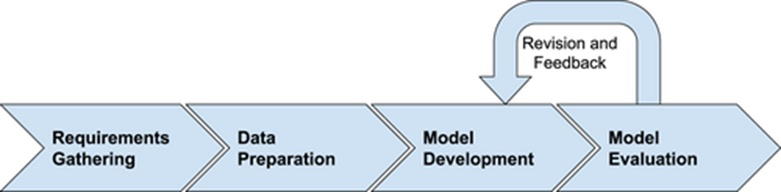
Figure 1. An abbreviated representation of the engineering lifecycle required for intelligent systems as outlined by Amershi et al. [5]. Their full machine learning workflow spans nine sequential phases: defining model requirements, acquiring data, refining data quality, annotating data points, extracting features, executing model training, verifying model performance, launching production deployment, and conducting continuous system monitoring [5].
While tech giants like Microsoft and Google possess the massive capital required to maintain in-house ML research, scaling AI across the broader economy depends on non-software organizations utilizing off-the-shelf DL systems to resolve their immediate operational bottlenecks. Public sector infrastructure stands to benefit immensely from this technological shift; the European Commission highlights that automated AI systems can provide citizens with continuous, around-the-clock service via faster, more adaptive, and highly accessible public channels [7].
A public utility organization central to this research partnership is the Metropolitan Sewer District of Greater Cincinnati (MSDGC) [8-11]. This collaborative initiative explores how DL frameworks can accurately anticipate combined sewer overflows (CSOs)—an environmental hazard ranked by the U.S. Environmental Protection Agency (EPA) as the single most critical unaddressed public health threat tied to modern water infrastructure [12]. Throughout the 2010s, MSDGC pioneered localized telemetry networks by implementing a SCADA (supervisory control and data acquisition) infrastructure. This network records dense historical data, such as logging in-pipe water elevations at 5-minute intervals. Converting this massive dataset into reliable, predictive intelligence presents an ideal opportunity to exploit DL capabilities.
Like many public infrastructure operations outside the software sector, MSDGC favors benchmarking existing DL models to rapidly gauge the feasibility, financial viability, and engineering trade-offs of these technologies. Requirements engineering (RE) is foundational to determining whether an algorithmic model is structurally fit for purpose. Practical deployment shows that a DL model's accuracy in forecasting overflow events cannot be evaluated in a vacuum; it must be stress-tested against the specific data failures that occur within the physical monitoring environment. For instance, our previous research evaluated how resilient these models remained when confronting data omissions caused by sensor dropouts [10], and explored how the mathematical stationarity of MSDGC’s multi-variable time-series feeds impacted overall neural network stability [8].
Rather than analyzing individual data anomalies in isolation, this study introduces a unified framework that binds data specification requirements directly to DL architectures using Jackson’s transformation problem frame [13]. Problem framing dictates that RE models must remain bound to verifiable, physical realities—a constraint we view as essential for diagnosing data anomalies and checking model validity. This work expands upon our earlier papers by offering a comprehensive validation strategy for MSDGC's forecasting goals, while explicitly detailing the operational compromises inherent to DL systems.
The core value of this study centers on utilizing the transformation problem frame to conduct a structured evaluation of how DL fits into MSDGC’s overflow mitigation strategies. By bridging problem framing with data specifications, this methodology provides a practical pathway for operators to better satisfy their engineering objectives.
Roughly 860 municipalities across the United States operate combined sewer infrastructures designed to collect both urban stormwater runoff and municipal wastewater within the same conduit network. Documentation from the EPA [12] indicates that approximately 850 billion gallons of this untreated wastewater escape into public waterways every year across the country. Major storms wash surface dust, municipal litter, and environmental debris from developed areas directly into these combined lines. When the volume of storm input overwhelms system capacity, the excess untreated sewage discharges directly into local rivers and streams via dedicated outfall structures, triggering a combined sewer overflow (CSO). This phenomenon occurs when internal water volumes scale past a conduit's maximum transport thresholds.
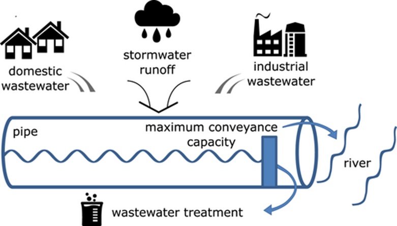
Figure 2. A visual depiction of an active overflow point, demonstrating the mechanism by which surges bypass standard treatment pathways and enter local aquatic environments.
Across the United States, the network of more than 9,000 active outfall locations causes roughly 5,000 public health infections annually, while destroying wetland habitats, causing major fish kills, and forcing the closure of public beaches and recreational waters [12]. The U.S. EPA characterizes this issue as the primary unresolved threat to human health across national water systems. This challenge is mirrored worldwide; for example, London’s River Thames receives an average annual influx of 39 million tons of raw sewage solely due to combined system overflows [14]. Similarly, rapidly modernizing metropolitan areas utilizing combined networks, such as Shenzhen, China, actively contend with heavy river pollution linked to these discharge events [15]. As urban density accelerates and global climate shifts intensify storm severity, these structural failures are projected to worsen, demanding automated, predictive solutions [14].
MSDGC oversees a service footprint spanning roughly 300 square miles, supporting more than 850,000 residents via a 3,000-mile network of combined sewer mains. Beginning in 2014, MSDGC deployed extensive sensor arrays across its most active watershed. Today, this monitoring network covers the vast majority of its service region, linking two major water reclamation facilities, six wet-weather containment and treatment installations, four large interceptor lines, 164 active discharge points, and 32 regional rain gauges and river telemetry stations [12]. This remote tracking system has optimized wet-weather facility management and allowed upstream systems to dynamically adjust for downstream interceptor constraints, maximizing overall basin containment during heavy rain.
Our research narrows focus onto a single, critical outfall location within MSDGC’s network. The operational dataset is derived from multiple telemetry devices, including sensors mounted within a utility manhole located roughly 450 feet upstream from the discharge gate, paired with a localized rainfall sensor. The system flags an active 'overflow state' whenever water levels exceed maximum holding limits. The manhole units record metrics continuously at 5-minute steps, as structured in the format of the first data layout. Concurrently, the second Table provides a simulated view of the precipitation sensor's minute-by-minute tracking cadence.
Table 1. A structured breakdown modeling the chronological telemetry captured from the upstream manhole junction, reflecting a recording frequency of one entry every 5 minutes.
Timestamp | … | Flow (ft3/sec) | Velocity (ft/sec) | Level(ft) | … |
… | |||||
Day1 13:35 | … | 0.07 | 0.70 | 545.21 | … |
Day1 13:40 | … | 0.10 | 0.09 | 545.87 | … |
Day1 13:45 | … | 0.09 | 1.08 | 546.79 | … |
… | |||||
Table 2. A simulated dataset reflecting rainfall intensity captured at 1-minute intervals, quantifying regional precipitation depth upstream of the primary discharge point.
Timestamp |
… |
Day1 13:33 |
Day1 13:34 |
Day1 13:35 |
Day1 13:36 |
… |
MSDGC's historical approach to predicting upcoming overflow events relies on analyzing standard regional weather forecasts and issuing public advisories if a spill appears likely within a 24-hour window. While utilizing regional weather forecasts offers a defensible justification for public notices, it produces a high rate of false alarms. Consequently, residents frequently become desensitized and ignore these alerts. Mitigating these systemic false positives is the primary driver behind exploring automated DL alternatives.
Successfully deploying DL models to achieve reliable overflow forecasts requires a deep understanding of the client organization's operational realities. To address this, we introduce the architectural framework structured in Figure 3, highlighting requirements engineering (RE) methodologies that clarify software development challenges [13] and organize data analysis through problem framing. Moving beyond the generic AI development lifecycle outlined in Figure 1, this methodology introduces structured mechanisms to embed domain expertise directly into the software development process.
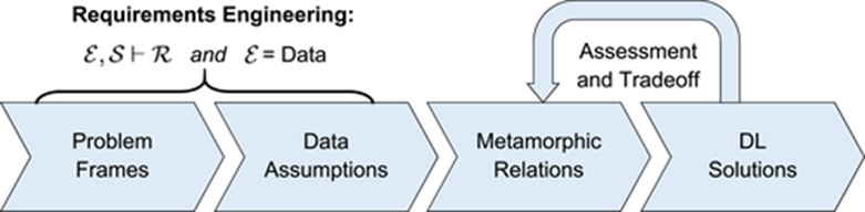
Figure 3. The structural methodology designed to check whether deep learning models satisfy practical operational demands. In contrast to standard machine learning workflows, this architecture prioritizes requirements engineering activities: structuring the software challenge, analyzing underlying data biases, and establishing automated testing protocols via metamorphic relations (MRs) to benchmark alternative DL models.
A primary deliverable generated by these RE activities is a suite of metamorphic relations (MRs) [16], which convert abstract data quality assumptions into concrete, testable validation code [17]. Merging RE analytical structures with automated neural network testing is a core innovation of our methodology. The MRs derived through this process yield a systematic framework for benchmarking diverse DL implementations. The following sections explore the first three modules of this validation architecture, followed by an analysis of the empirical testing results.
Jackson’s problem frames methodology in software engineering emphasizes analyzing the problem space itself rather than jumping straight to solution design [13]. Since practical engineering challenges are typically complex, Jackson's method provides structural abstractions—problem frames—to decompose an overarching problem into a network of interacting subproblems. Each subproblem is more compact, less complex, and easier to understand, possessing clearly defined interfaces. This conceptual abstraction serves as the foundation for transitioning from initial problem detection to systematic problem structuring.
Problem frames function as analytical instruments that help crystallize the precise intent of software requirements [18]. Figure 4 outlines Jackson’s foundational requirements engineering principle [18], where a deep learning (DL) machine that implements a specific machine specification S, when deployed within an operational environment characterized by environmental assumptions W, must successfully achieve the stakeholder requirements R, expressed as W, S \vdash R. Within the context of MSDGC, the core requirement evaluated is the capacity to ‘manage CSOs ahead of the time’. As previously noted, MSDGC’s historical strategy relies on issuing public notifications regarding potential CSO risks 24 hours in advance by evaluating regional meteorological forecasts. Developing the capability to generate predictions across multiple temporal windows (such as 24, 12, or 2 hours prior to an overflow event) provides MSDGC with diverse operational alternatives to handle incoming events proactively (e.g., executing area-specific citizen alerts, deploying field crews to specific sites, etc.).
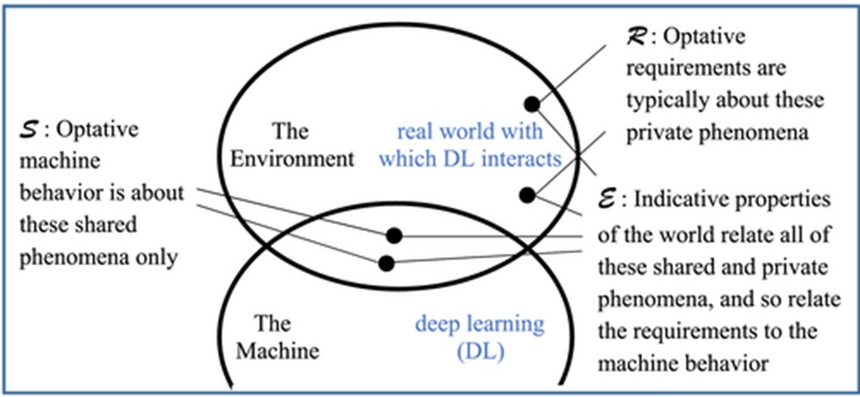
Figure 4. A DL solution implementing the machine specification S, once installed in the environment having properties of W, shall satisfy the stakeholder requirements R. Such an entailment relation, W, S \vdash R, defines the meaning of requirements [18].
Isolating the requirement of ‘managing CSOs ahead of time’ directs our attention toward the transformation frame to map out the structure of the problem. Figure 5 illustrates this specific problem frame, where the proposed DL framework essentially processes the input domain—comprising sensor network streams and precipitation data (Tables 1 and 2)—to produce outputs in the destination domain of CSO predictions. As shown in Figure 5, the destination domain is directly bounded by the operational requirement, whereas the input domain remains unconstrained. The internal mechanics of the DL machine, while generating these overflow forecasts, are fundamentally driven by the diverse data streams originating from the input domain.
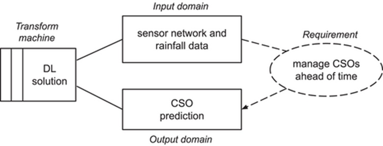
Figure 5. DL-based CSO prediction framed as a transformation problem [13]: the to-be-built transform machine (a box with a double stripe) interfaces with (a solid line) the given input and output domains (boxes with no stripe) in order to satisfy the requirement (a dashed oval). A dashed line is a requirement reference, whereas a dashed arrow is a constraining requirement reference [13].
The transformation problem frame does more than simplify our understanding of how DL operates within CSO forecasting; it also provides a structured foundation for validating the entailment relation W, S \vdash R. This validation is pursued by tracking the core interactions across the frame. In a transformation problem, Figure 6 shows that as the software machine simultaneously processes the input and output domains, it computes the appropriate values to populate the destination domain based on the real-time data values encountered within the source domain [13]. This structural traversal continuously aligns with the organization and data properties of both the input and output domains, thereby ensuring that the overarching requirement is fulfilled.
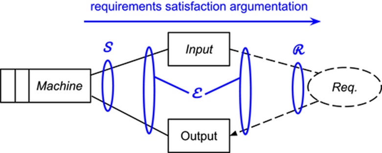
Figure 6. Frame concerns in the transformation problem where the requirements satisfaction argumentation traverses from the machine specifications S, through the environmental assumptions W, towards requirements fulfilment R [18].
To illustrate, a DL model designed for overflow prediction must accept data streams from both the in-pipe sensor network and precipitation logs across differing temporal sampling rates, ultimately outputting the probability of a future overflow incident. These mechanisms form the core of the machine behavior specification S. The physical environment, W, is characterized by multivariate time-series data feeds as inputs, yielding time-critical overflow predictions as outputs. Maintaining these simultaneous input-output behaviors over S will logically lead to satisfying the requirement R, thereby empowering MSDGC to make proactive management decisions prior to overflow events.
It is worth noting that transformation represents just one of five distinct problem frames established by Jackson [13], alongside required behavior, commanded behavior, information display, and simple workpieces. While the transformation frame is ideal for the objective of managing CSOs ahead of time, separate operational requirements—such as ‘monitoring CSOs in real time’—would be better served by an alternative frame, such as information display. Shifting to a different frame would fundamentally alter the underlying problem architecture and the corresponding validation traversal process.
Decomposing the problem space through problem frames, as depicted in our core methodology in Figure 3, allows for a transparent and explicit analysis of underlying data assumptions. When we evaluate data assumptions, we specifically focus on the input domain, treating W as a set of indicative characteristics that reflect real-world conditions independent of the specific software machine being designed (Figure 4). Because DL networks are uniquely capable of operating directly on raw environmental observations to construct their own internal features for predictive tasks [19], data effectively serves as the core environment for a DL system. Consequently, the environmental assumptions surrounding a DL model translate primarily into assumptions regarding its data.
Jackson’s emphasis on anchoring requirements engineering abstractions directly to observable physical phenomena [13] is essential for interpreting these data assumptions. For MSDGC’s input domain, Figure 7 FIGUREs the physical dynamics occurring within the specific problem environment of overflow forecasting. The conduit illustrated in Figure 7 features a downward gradient terminating at an exit gate that leads to a wet-weather retention basin before merging with subsequent lines routed toward the wastewater treatment plant. Within this conduit, the flow sensor is anchored at the invert (bottom), positioned upstream of the water level sensor mounted near the crown (top). For visual clarity, the regional precipitation monitoring gauge is omitted from Figure 7.
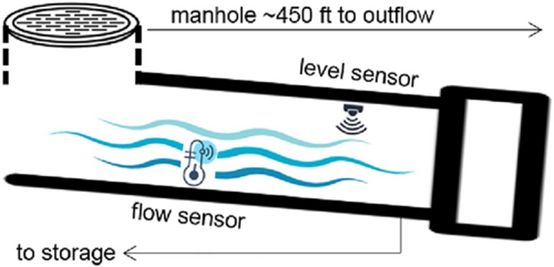
Figure 7. Input domain phenomena that are part of W in Figure 6's frame concerns.
When the telemetry network and precipitation feeds are aggregated within the input domain as shown in Figure 5, we establish baseline assumptions regarding these data assets to construct our DL models. Our expectations for high-quality data properties align with established industry frameworks such as ISO/IEC 25012 [20]. As categorized in Figure 8, data quality dimensions are split into two major perspectives: inherent characteristics and system-dependent properties. In the second stage of our methodology, which addresses data assumptions, we restrict our focus to inherent quality features. This is because system-dependent metrics, such as availability and recoverability, are determined by how the software architecture preserves data and governs access.
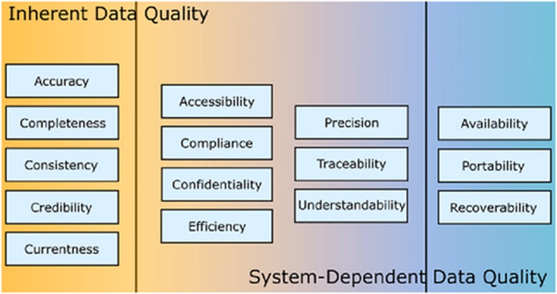
Figure 8. Inherent data quality includes: accuracy, completeness, consistency, credibility, and currentness (adopted from [20]).
While the five inherent data characteristics listed on the left side of Figure 8 apply broadly across diverse media types (such as imagery or unstructured text), our framework operates by anchoring and contextualizing these traits directly within the physical input domain illustrated in Figure 7. Using Figure 8 as an analytical guide, we map our targeted data quality expectations directly to the real-world physical dynamics shown in Figure 7.
This mapping is detailed in Table 3. Notably, certain inherent quality dimensions from Figure 8 are less relevant within MSDGC's unique operational context. For example, credibility—which evaluates data authenticity, including the validity of origins, tracking, and source commitments [20]—exerts minimal impact on the operational performance of overflow forecasting. Conversely, as demonstrated in our previous investigations [8], stationarity is a defining feature of time-series feeds and is therefore integrated into Table 3. Conceptually, a time-series dataset achieves stationarity when its underlying statistical metrics, such as mean values and correlation coefficients, remain constant over time [21].
Table 3. Using input domain's phenomena to analyse data assumptions.
Data Quality Dimension (Desired Characteristic) | Underlying Data Assumption (Potential Source of Error) |
Accuracy | The transport of coarse solid materials may occasionally generate anomalous Velocity measurements, resulting in outlier values. |
Completeness | Flow observations may intermittently be unavailable because of the influence of bedload transport processes. |
Consistency | The sampling intervals differ across variables: Rainfall measurements are recorded every 1 minute, while Flow, Velocity, and Level are collected every 5 minutes. |
Currentness | The presence of suspended sediment transport can introduce delays in the transmission of Level measurements. |
Stationarity | Owing to the downward channel gradient and local storage effects, increases in Flow and Velocity do not necessarily coincide with corresponding increases in Level. |
Table 3 outlines both our optimal data quality expectations and the specific environmental conditions where these underlying data assumptions are vulnerable to failure. These vulnerabilities are tied directly to hydrological occurrences, including the movement of gross solids, bedload displacement, and the migration of suspended sediment. Furthermore, sensor sampling frequencies and network topology configurations represent foundational factors in this evaluation. The data assumptions structured in Table 3 explicitly define the environmental conditions W within the input domain of our transformation problem frame. Because W represents an indicative description of reality, any candidate DL model must be engineered to account for these specific data assumptions.
The third phase of our methodology involves establishing metamorphic relations (MRs) as software verification benchmarks for the identified data assumptions (cf. the right-hand column of Table 3). The generated MRs can subsequently be employed to quantitatively evaluate diverse DL solutions, as FIGUREmed in Figure 3. MRs represent indispensable behavioral attributes of the software under review, which are applied within the metamorphic testing paradigm [16] to circumvent the challenge of missing test oracles. For instance, determining the precise numerical value of the trigonometric function sine(x) may be impossible due to floating-point computations and rounding decisions within a specific implementation. This inability to verify the exact anticipated output of sine(x) illustrates the test oracle problem.
Metamorphic testing utilizes MRs to mitigate this test oracle limitation. An illustrative MR for the sine function is sine(x) = sine (π − x), which represents an invariant attribute of this trigonometric operation. By leveraging this MR, software testing can proceed by executing the code across two distinct steps: initially with a source test input, such as sine (12), and subsequently with a follow-up test input, namely sine (π − 12). Investigators can then verify whether the output of sine (12) equals the output of sine (π − 12) without requiring prior knowledge of the exact numerical oracle for either calculation. Since MRs define essential behavioral properties, any failure in these relationships confirms that the underlying software contains a fault [22].
When transitioning MRs to ML systems in general and DL frameworks in particular, these properties are frequently treated as expected objectives rather than absolute invariants. This distinction arises from the structural ambiguity and stochastic nature characteristic of DL models [17]. To illustrate, an MR presented in the foundational research by Murphy et al. [23] relies on permutation; specifically, reordering the elements of the input dataset should leave the overall ML model performance largely stable, even if minor output fluctuations (e.g., classification precision) occur during operations like n-fold cross-validation. Consequently, MRs designed for a DL machine represent target properties where compliance is measured along a spectrum rather than as a strict binary success-or-failure outcome.
To predict upcoming CSOs, we analyze a family of DL frameworks built upon the recurrent neural network (RNN) architecture. Figure 9 demonstrates the standard RNN paradigm where node interconnections establish a directed graph across a temporal sequence, enabling the DL system to model time-dependent dynamic behaviors. This architectural selection aligns with the methodologies of Zhang, where RNNs were trained to forecast stormwater runoff using precipitation variables and historical discharge values [24]. In Figure 9, the temporal axis is unfolded horizontally; hence, xt−1, xt, and xt+1 denote the input patterns at time steps t - 1, t, and t + 1, respectively. Correspondingly, ot−1, ot, and ot+1 represent the generated outputs at those respective steps. The variables U, V, and W represent the structural weight matrices, while h designates the hidden layer state. We utilize E(t) to represent the backpropagated loss metric [25] at time step t.
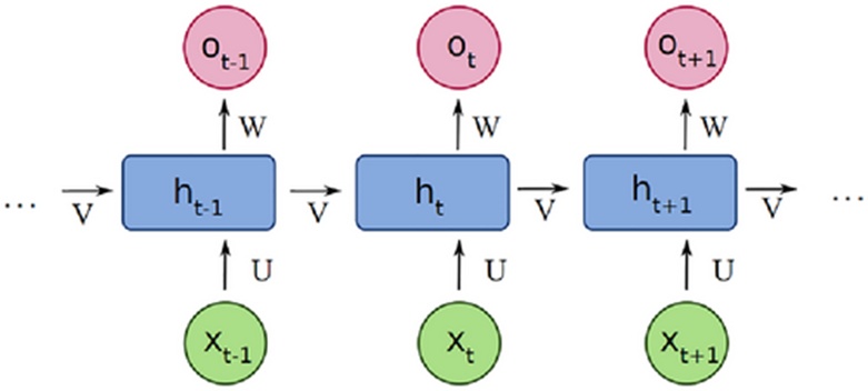
Figure 9. Architecture of a recurrent neural network (RNN) for making time series predictions (adopted from https://en.wikipedia.org/wiki/Recurrent_neural_network).
As demonstrated by the expression sine(x) = sine (π − x), every MR is composed of two primary elements: (1) an input modification that maps a source test case to a subsequent follow-up test case, and (2) an output comparison relation that validates the outputs generated by this pair of test cases [16]. Within our framework, the input modification is derived directly from the physical data assumptions. We outline below the verifiable MRs designed to mirror the data assumptions structured in Table 3.
Accuracy: To address 'Velocity' anomalies, the source test case is selected from sequential time increments where E(t - 1) > E(t), signifying that the prediction error at step t is lower than at step t - 1. Stochastic noise is then introduced into the 'Velocity' metric at step t to replicate an anomaly-driven distortion. This perturbation generates the follow-up test case, designated as t'. The target MR is formulated as E (t′ − 1) ≤ E (t′), capturing the expected increase in prediction error caused by the artificial anomaly.
Completeness: We have previously engineered a dedicated MR to manage missing 'Flow' telemetry [10]. The source test case identifies three sequential time increments satisfying E (t − 1) ≥ E(t) ≥ E (t + 1), which demonstrates a pattern of decreasing error under nominal data conditions. The follow-up test case substitutes the real xt value for 'Flow' with the prior output ot−1, simulating a telemetry dropout at step t. Following this modification at step t', the MR expects that E(t' - 1) ≥ E(t' + 1) in the subsequent execution, thereby validating resilience against missing 'Flow' data.
Consistency: Discrepancies in data gathering frequencies are evaluated based on how precipitation records are scaled upward from a 1-minute cadence to a 5-minute window. Given that the operational goal is to anticipate overflow events, the source test case uses the maximum recorded precipitation value across each 5-minute interval. The follow-up test case executes alternative aggregations, such as mean, median, mode, or minimum values. For this validation, the follow-up test case employs the mathematical average, and the target MR is defined as E(t) < E(t'), establishing that prediction errors are minimized when using peak values rather than averages.
Currentness: Data latency is modeled by maintaining the 'Level' input recorded at step t as a constant value across the subsequent m time intervals (where m = 3 in this study). This frozen 'Level' feed spanning from t' to t' + m constitutes the follow-up test case. When contrasted with the baseline source test case that lacks transmission delays, the MR expects an accumulation of backpropagated errors across the delayed interval, expressed mathematically as \sum_{\tau=t'}^{t'+m} E(\tau) > \sum_{\tau=t}^{t+m} E(\tau).
Stationarity: To evaluate stationarity characteristics where the 'Level' metric might deviate from trends observed in 'Flow' and 'Velocity', a linear function is applied to construct the follow-up test case [8]. Specifically, the transformation is defined as x'_{t,\text{Level}} = (\alpha \cdot x_{t,\text{Level}} + \beta) / \gamma exclusively for the 'Level' attribute, utilizing parameters α = 2, β = 1, and \gamma = 3. This metamorphic stationarity adjustment is grounded in the principle that altering the variance of a single parameter within a multivariate time series disrupts the underlying stationarity of the dataset. The anticipated consequence of this statistical disruption yields the MR expressed as E(t) < E(t').
Although our earlier research explored MRs isolated to completeness [10] and stationarity [8], the consolidated framework FIGUREmed in Figure 3 permits a comprehensive and systematic derivation of MRs anchored directly to observable physical phenomena within the problem domain. While the data assumptions characterize the physical challenges impacting the input domain, the MRs balance this analysis by specifying the target behavioral properties of the output domain. Because the transformation problem frame tracks both the input and output domains concurrently to construct a requirements validation argument (Figure 6), these MRs—combining an input transformation with a corresponding output relation—offer a systematic methodology to evaluate whether a DL engine is fit for purpose.
To evaluate the practical utility and performance of our proposed framework, we conducted an exploratory case study [26]. This investigation analyzes the real-world dynamics of contemporary CSO events within their operational context, focusing on three core research questions (RQs):
RQ1: Are the MRs derived from our RE activities suitable for the problem context?
MRs define the software testing benchmarks crucial for evaluating competing DL systems. We address RQ1 by reviewing published literature regarding MR applications in ML and DL domains, followed by an analytical assessment of their suitability for MSDGC's unique operational constraints.
RQ2: Do the MR operations derived from the physical observables provide proper DL comparisons?
Our RE process defines both the verifiable MR properties and the optimal execution strategy for each relation. For instance, testing completeness does not merely involve replacing x_t with o_{t-1} generically, but requires applying this substitution specifically to the 'Flow' attribute rather than other variables. We address RQ2 by quantitatively comparing the software testing outcomes of MRs executed according to our framework against identical MRs executed using alternative configurations.
RQ3: What are the pros and cons of different DL solutions?
A core practical benefit of our methodology is providing utility operators, such as MSDGC administrators, with clear insights into the technical trade-offs of competing DL models when balancing diverse and occasionally conflicting operational needs. We address RQ3 by constructing a softgoal interdependence graph (SIG) [27] derived from our empirical MR testing, where requirements fulfillment levels are modeled via positive or negative softgoal contributions.
We conducted a comprehensive review of existing literature focusing on MR implementations for ML and DL frameworks, identifying five primary studies categorized in Table 4. The majority of these investigations target standard ML environments, though Ding and colleagues [28] specifically evaluated DL models. While most tasks involve supervised learning configurations, Xie et al. [29] also explored unsupervised methods (i.e., cluster analysis). In contrast to the relatively uniform learning tasks and domains, the underlying data structures exhibit greater heterogeneity, spanning imagery, synthetic numerical records, and spiral geometric formations.
Table 4. Studies on metamorphic relations (MRs) for machine learning (ML) and deep learning (DL) applications.
Study | Study Context | Metamorphic Relation (MR) Characteristics | ||||||||
Application Domain | Analytical Task | Type of Data | Total Number of MRs | Accuracy | Completeness | Consistency | Currentness | Stationarity | Applicable MRs | |
Dwarakanath et al. [30] | Retail sector | Forecasting sales for the following day | Pricing and commodity information | 19 | 1 | 1 | 1 | 0 | 0 | 3 (16%) |
Xie et al. [29] | Machine learning | Clustering and classification analysis | Artificially generated numerical data | 10 | 1 | 1 | 0 | 0 | 0 | 2 (20%) |
Zheng et al. [31] | Machine learning | Classification using neural networks | Synthetic spiral datasets | 6 | 0 | 0 | 0 | 1 | 0 | 1 (17%) |
Dwarakanath et al. [32] | Machine learning | Image recognition and classification | Generic image datasets | 5 | 0 | 0 | 1 | 0 | 0 | 1 (20%) |
Ding et al. [28] | Deep learning | Image classification | Biological cell image data | 11 | 1 | 0 | 0 | 0 | 0 | 1 (9%) |
Σ | -- | -- | -- | 51 | 3 | 2 | 2 | 1 | 0 | 8 (16%) |
The metamorphic relation statistics presented in Table 4 detail the overall volume of MRs established within each investigation, further breaking down the specific count of MRs relevant to the five core data assumptions of combined sewer overflow forecasting. As indicated by Table 4, a maximum of 20% of the MRs documented across existing literature prove compatible with MSDGC’s specific operational problem space. This accentuates the profound impact that the unique domain context exerts on the usability of metamorphic relations.
Among the compatible benchmarks, three focus on data accuracy: their follow-up evaluations introduce anomalous spikes [30], apply arbitrary affine coordinate transformations [29], or delete an entire category from the underlying image data [28]. The two relations addressing data completeness inject missing data points [30] or introduce non-informative parameters [29] into their respective follow-up evaluation cycles. The consistency-related benchmarks both rely on executing linear scaling adjustments on feature magnitudes [30, 32]. Network latency impacting data currentness is simulated within the follow-up cases by multiplying any pair of features by a factor of 1–10 times [31]. Crucially, the compatible MRs extracted from these five reviewed studies remain highly abstract. Furthermore, no metamorphic relation has been designed to evaluate dataset stationarity, which is an indispensable attribute of multivariate time-series feeds [21]. These structural evaluations provide the following resolution to RQ1:
Discerning the environmental context is essential for MR viability, as merely a minor portion of the metamorphic relations reviewed in the literature could be practically deployed. Conversely, the specific MRs engineered via our requirements engineering framework yield far superior alignment.
To resolve RQ2 and RQ3, we evaluated three distinct RNN designs, all of which align with the network topology FIGUREmed in Figure 9. We engineered a long short-term memory (LSTM) architecture based on Ref. [33] featuring four hidden layers configured with 128 neurons each. We selected the 'ReLU' activation function for each network layer, updated the model using the 'Adam' optimization algorithm, calculated training errors (the loss function) via 'mean square error', established a learning rate of 1e-3, and executed model training for 30 epochs utilizing a batch size of one to generate the CSO forecasts. Our second RNN variant was a gated recurrent unit (GRU) designed on top of [33]. This GRU setup matched the exact structural parameters utilized in the LSTM variant regarding hidden layer configuration, activation functions, optimization routines, loss metrics, learning rates, epoch durations, and batch sizes. Our third RNN configuration was an independent recurrent neural network (IndRNN) structured on a conventional fully connected network. We developed this IndRNN based on Ref. [34], utilizing three hidden layers of 128 neurons each. For the IndRNN model, we chose the 'ReLU' activation function, the 'Adam' optimizer, and the 'categorical cross entropy' metric to determine the training loss. We configured its learning rate to 1e-3 and completed model training over 30 epochs with a batch size of one.
Since RQ2 isolates the variation between running MR operations tailored to the physical dynamics dictated by our methodology and running those identical MRs via alternative configurations, we tested 2 specific MR variants: one focusing on dataset accuracy and the other on data completeness. For the accuracy-based MR, our domain analysis dictated that the follow-up validation step at increment t should introduce a random disturbance exclusively into the 'Velocity' parameter to simulate the gross solid transport dynamics detailed in Table 3. Across a cumulative pipeline of 24,116 baseline test executions, the proportion of successful follow-up outcomes under the 'Velocity' disturbance configuration reached 85.50%, 73.58%, and 84.34% for the LSTM, GRU, and IndRNN architectures, respectively. In contrast to our framework's structured logic, if a random disturbance is instead introduced into the 'Flow' and 'Level' parameters, the resulting validation success rates for the LSTM, GRU, and IndRNN models shift to 95.35%, 94.30%, and 95.57%, respectively. Figure 10 maps out these behavioral fluctuations. While our structured approach exposes stark performance variances among the diverse RNN designs, altering the MR application points produces uniform software testing metrics that obscure these differences, potentially misguiding the benchmarking of DL architectures.
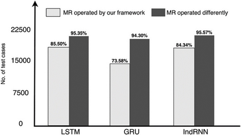
Figure 10. Test case pass rates when the accuracy MR is operated on ‘Velocity’ as defined in our framework compared with when this MR is operated on the different sensor network data: ‘Flow’ and ‘Level’ (total # of test cases: 24,116).
The completeness-oriented MR demands three consecutive temporal steps. Furthermore, the baseline test pattern must strictly satisfy the inequality condition E(t - 1) ≥ E(t) ≥ E(t + 1). Consequently, we isolated a total of 8,500 qualified evaluation patterns for this completeness test suite. Table 3 specifies that the 'Flow' parameter must be adjusted in the follow-up test pattern to substitute the real input xt with the prior output state ot−1. This exact execution strategy yields validation success rates of 71.56%, 57.48%, and 70.90% for the LSTM, GRU, and IndRNN models, respectively, as illustrated in Figure 11 and documented in Ref. [10]. However, if this identical MR is deployed against alternative data attributes like 'Velocity' and 'Level', the recorded success benchmarks shift to 49.16% for LSTM, 73.21% for GRU, and 30.24% for IndRNN. Following our framework’s 'Flow'-centered protocol reveals that LSTM and IndRNN achieve comparable validation success rates, both significantly outperforming the GRU model. Manipulating the MR differently creates an inverse illusion where the GRU appears superior to both the LSTM and IndRNN networks. Guided by the empirical metrics visualized in Figures 10 and 11, we formulate the following response to RQ2:
Even when metamorphic relations are fundamentally compatible with the operational environment, executing them in alignment with core physical phenomena yields significantly more meaningful and precise comparisons of DL architectures.
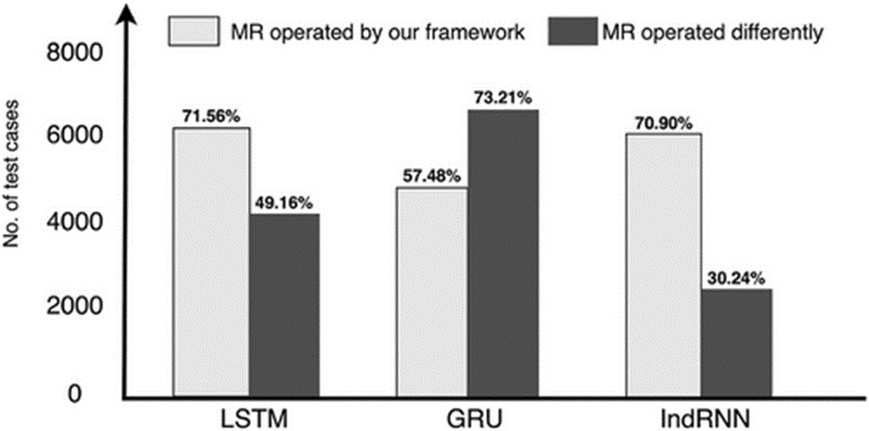
Figure 11. Test case pass rates when the completeness MR is operated on ‘Flow’ as defined in our framework compared with when this MR is operated on the different sensor network data: ‘Velocity’ and ‘Level’ (total # of test cases: 8500).
Having verified the parameters for MR suitability and operational precision, we leverage these metamorphic relations to execute automated evaluations across the three RNN frameworks. Figure 12 provides a series of radar visualizations mapping out validation success benchmarks across all five analytical axes: accuracy, completeness, consistency, currentness, and stationarity. These radar charts visually clarify how effectively each deep learning engine navigates competing requirements when translating raw data into overflow predictions.
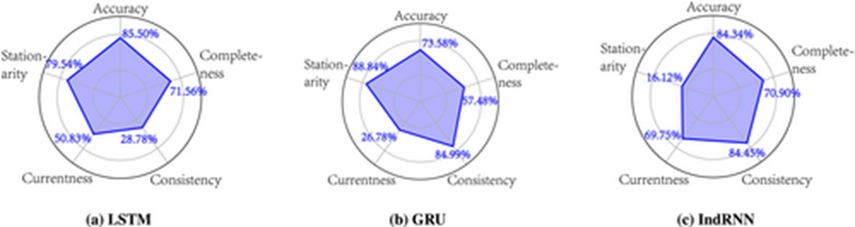
Figure 12. Using the MRs to assess the degree to which the DL solutions meet the accuracy, completeness, consistency, currentness, and stationarity data requirements. Each dimension plots the percentage of passed test cases.
All three recurrent network variants achieve a validation success rate exceeding 50% across four of the tested dimensions, illustrating the baseline competence of these DL models. However, individual network topologies expose unique vulnerabilities: the LSTM architecture satisfies only 28.78% of consistency test scenarios, the GRU system achieves just 26.78% success on currentness benchmarks, and the IndRNN architecture drops to a 16.12% success rate regarding stationarity parameters. These deficiencies indicate that none of the examined deep learning frameworks can perfectly satisfy all data constraints simultaneously.
To break down the operational trade-offs governing these diverse data criteria, we construct the softgoal interdependence graph (SIG) illustrated in Figure 13. Within this SIG, the primary engineering objective of reliable CSO forecasting is broken down into five underlying sub-goals, each of which is satisfied to varying degrees [27]. Positioned at the bottom of the SIG structure are the target DL models, with each link representing either a supportive or obstructive contribution to the defined softgoals. Capitalizing on the automated, quantitative evaluations driven by our MR framework, we convert raw validation success percentages into the qualitative evaluation categories of break (--), hurt (−), help (+), and make (++). As shown in Figure 13, both the accuracy and completeness parameters secure positive validation contributions, proving that these DL frameworks possess strong resilience against noisy data anomalies and data omissions. Conversely, data currentness emerges as the most volatile operational dimension; the LSTM and GRU implementations contribute negatively to this goal, while the positive contribution from the IndRNN engine reaches only the (+) tier. This demonstrates that although recurrent models can successfully learn to anticipate overflow events by caching historical patterns, encountering stale data inputs introduces a major performance bottleneck for the DL architectures evaluated. Our structural investigation of RQ3 yields the following conclusion:
Recurrent neural network models exhibit robust performance metrics across the five core data dimensions, yet none of the three evaluated RNN frameworks yields exclusively positive contributions. Managing stale data inputs—as opposed to coping with noisy or omitted metrics—represents a critical challenge demanding advanced RNN architectural innovations.
![Figure 13. Softgoal interdependence graph (SIG) for the DL machines. The undirected lines represent goal decompositions, and the arrows represent softgoal contributions [27]: ‘--‘ means ‘breaks’ where the test case pass rate is less than 25%, ‘-’ means ‘hurts’ where the test case pass rate is in [25%, 50%), ‘+’ means ‘helps’ where the test case pass rate is in [50%, 75%), and ‘++’ means ‘makes’ where the test case pass rate is greater than or equal to 75%.](https://pubsys.eshragh.co/storage/files/pub-article/a7735d2f-b0e0-44e0-827d-0fc9a5bf0e40-ilhmvu6sCRiSN9o3/image.jpg)
Figure 13. Softgoal interdependence graph (SIG) for the DL machines. The undirected lines represent goal decompositions, and the arrows represent softgoal contributions [27]: ‘--‘ means ‘breaks’ where the test case pass rate is less than 25%, ‘-’ means ‘hurts’ where the test case pass rate is in [25%, 50%), ‘+’ means ‘helps’ where the test case pass rate is in [50%, 75%), and ‘++’ means ‘makes’ where the test case pass rate is greater than or equal to 75%.
A primary threat to construct validity centers on the fact that different metamorphic relations require highly variable totals of applicable test patterns. For example, as plotted in Figures 10 and 11, the absolute volumes of qualified evaluation patterns stand at 24,116 and 8,500, respectively. To account for these systemic variances, Figure 12 uses percentage scaling to normalize the underlying evaluation constructs, an adjustment that must be kept in mind when evaluating the analytical findings.
We argue that the internal validity of this study remains exceptionally high because all operational variables capable of altering the test validation success thresholds were maintained under our direct experimental control. This isolation ensures that the selected MR properties and their exact execution setups function as the direct causal drivers of the observed performance variations.
Regarding external validity, our empirical findings may not directly generalize to alternative RNN variants or broader deep learning architectures. One specific boundary condition to note is that our team engineered a single metamorphic relation to represent each data quality requirement. While each relation was systematically derived via problem space modeling rooted in physical observables, a larger array of MR configurations could potentially be formulated for these identical data characteristics [35]. Furthermore, it remains possible that certain data quality dimensions omitted from this study may not map cleanly to metamorphic validation structures. Nonetheless, this exploratory case study focusing on MSDGC's overflow prediction challenges confirms the utility, validity, and viability of our requirements engineering framework for benchmarking alternative DL architectures.
We examine two distinct bodies of literature relevant to our study: the application of DL to water-management issues and the utilization of problem frames within industrial contexts.
Forecasting techniques based on DL are attracting substantial interest within waterworks and associated fields. Initial work by Zhang [24] was among the earliest to train an RNN for predicting stormwater runoff based on precipitation data and historical runoff discharge. Conducting experiments on a dataset consisting of 34,721 timesteps gathered from a CSO site near the District of Columbia, the study demonstrated that runoff forecasting achieved high accuracy when utilizing a hidden layer configured with 50 neurons. These highly accurate outcomes were realized by allocating 70% of the dataset (24,305 target time steps) for model training, 15% (5,208 target time steps) for validation purposes (improving network generalization and terminating training when performance gains plateaued), and the remaining 15% (5,208 target time steps) for testing [24].
In a similar vein to the investigation presented in Ref. [24], Kim and Han [36] leveraged DL techniques to forecast overflow using stormwater management model data. To boost the predictive capacity of their DL model, they introduced data augmentation strategies, specifically by injecting noise comprised of random numbers bounded between zero and one while preserving a Gaussian distribution. Their empirical testing utilized 6 hours of meteorological rainfall data sourced from the Korean Meteorological Administration (KMA) to project urban flooding, employing a DNN to generate predictions across 69 out of 70 distinct municipalities in South Korea. The findings indicated that these data augmentation techniques successfully decreased the mean absolute error (MAE) from 23.87 down to 4.46.
Beyond stormwater management, investigators have deployed DL architectures to project the outputs of water purification facilities over continuous time cycles. Cao et al. [37] integrated a convolutional neural network (CNN) to execute feature selection on inputs with an LSTM to handle time-series forecasting. A dataset spanning an entire year (comprising 132,480 time steps) was utilized to train the DL models, whereas a 7-day window of data (amounting to 10,080 time steps) served as the evaluation test set. For any designated temporal point ‘t’, the DL systems were constructed to project outputs for subsequent ‘t + 1’, ‘t + 2’, …, ‘t + n’ time steps. When encountering omitted observations within the sensor streams, the researchers substituted them with a value of ‘0’. The assessment revealed that utilizing the standalone CNN model yielded an average error of 132.1, the standalone LSTM model produced an average error of 104.7, and combining the CNN and LSTM architectures minimized the average error to 16.4.
An additional notable deployment of predictive DL architectures within water infrastructure was conducted by Du et al. [38]. The investigators used an LSTM network to project urban water demand volumes, utilizing a dataset of 1,660 daily water demand observations from Suzhou, China. The training partition comprised 998 daily observations, while the testing partition held 662 daily observations. Du et al. [38] leveraged the Discrete Wavelet Transform (DWT) to mitigate correlation friction between historical and current data, and further coupled DWT with principal component analysis (PCA) to decrease dimensionality prior to generating predictions with the LSTM.
The core objective of our study diverges from the aforementioned research. Rather than attempting to engineer a novel DL algorithm or boost predictive precision through data augmentation, we introduce an RE-driven framework. This framework is designed to contextualize problems within their real-world environments to analyze critical data assumptions and evaluate how effectively DL approaches resolve these challenges. Our investigation does not claim the superiority of any single DL algorithm; instead, it offers a trade-off analysis detailing which algorithms excel under specific criteria. Consequently, practitioners are equipped to assess, select, and refine DL applications through a structured methodology.
Problem frames serve as methodologies for evaluating and organizing software engineering challenges [13]. Strunk and Knight [39] implemented a problem frames perspective within a case study focused on interpreting aircraft runways. They utilized problem frames to formulate objectives and organize the operational context for assurance cases. They established context FIGUREs alongside an information display problem frame to model the runway environment and its function during aircraft landing and takeoff sequences. Our investigation draws inspiration from the approach of Strunk and Knight [39] regarding the interpretation of challenges from a physical-world perspective. We build upon their methodology by explicitly integrating the underlying data assumptions tied to the physical phenomena of the problem domain.
Han et al. [40] integrated goal-oriented models alongside problem frames to evaluate requirements for cyber-physical systems. Goal modeling served to establish high-level objectives, while problem frames were utilized to comprehend functional requirements and operations. This methodology was implemented during the engineering of a fire disaster alert system, where the primary objectives centered on monitoring fire events and deploying emergency countermeasures. The researchers utilized a variant of a requirements behavior frame to simulate an intelligent building firefighting architecture encompassing two distinct problem domains: fire sensors for monitoring purposes and emergency countermeasures for prompting the system to distribute water. The practical application demonstrated that problem frames successfully provided an appropriate context for established goals [40]. Although our CSO forecasting problem shares parallel monitoring characteristics, our study leverages the transformation problem frame to evaluate the requirements of DL architectures.
Yuan et al. [41] deployed problem frames to validate safety requirements within Communication-Based Train Control setups. Their methodology aligns closely with the required behavior and information display frames. The machine domain consisted of zone control verification software tasked with determining if safety constraints were satisfied. Upon successful verification, an analytical report was generated in accordance with the information display problem frame.
Wang et al. [42] utilized problem frames to structure the verification of timing requirements inside automated high-speed rail systems. They engineered two problem domains structured around a clock constraint specification language. Their configuration involved creating an interactive clock that synthesized time data from various sensors, alongside a domain clock where multiple interactive clocks could interface based on the underlying problem domain (such as wheels or brakes). Problem frames were employed to formulate these timing specifications. However, the researchers did not explicitly designate a specific problem frame, though their approach suggested the application of context FIGUREs rather than a strict behavior frame.
The previously reviewed literature indicates that problem frames have been utilized to evaluate diverse operational contexts and a variety of requirements (including sensing, monitoring, safety, and timing metrics). Capitalizing on these foundations, our research bridges the gap between problem frames and DL methodologies. To our knowledge, this framework represents the initial effort to couple problem analysis with solution assessment by utilizing data assumptions and MRs.
For a wide range of enterprises, including public sector entities, substantial opportunities exist to leverage the ongoing AI transition driven by DL. Nonetheless, the deficit of structured guidance for determining if a DL solution is fit for purpose acts as an impediment to adoption. In this paper, we introduced a framework that highlights RE tasks for organizing DL engineering via a transformation problem frame, while evaluating pivotal data assumptions tied to the framed physical phenomena. Our methodology subsequently connects these RE tasks through MRs to perform quantitative evaluations of DL systems. Our empirical case study focusing on MSDGC's CSO forecasting highlights both the practicality and the viability of the proposed framework. Specifically, we demonstrate the utility of the MRs established via RE tasks alongside the operational methodologies required for these MRs. Additionally, our framework yields observations regarding the comparative advantages and limitations of three distinct RNN variants: LSTM, GRU, and IndRNN.
There are multiple pathways for expanding this research. We plan to investigate alternative problem frames (such as information display) to address different dimensions of DL-driven CSO forecasting. Furthermore, we intend to broaden our analysis of data assumptions to encompass a wider array of criteria, including the system-dependent data quality properties illustrated in Figure 8, such as traceability [43] and availability [44]. It is important to note that MRs might not align with every data requirement, indicating opportunities for further framework optimization. Through more comprehensive case studies across varied domains alongside theoretical replications [45, 46], we expect that our refined framework will deliver valuable RE support and DL insights to user organizations across both public and private domains.
None
None
This research is partially funded by the National Natural Science Foundation of China (No. 62177003).
None
Open Access The author(s) retain copyright. This article is licensed under the Creative Commons Attribution-NonCommercial-ShareAlike 4.0 International License. It may be shared and adapted for non-commercial purposes with appropriate attribution, an indication of changes, and distribution of adaptations under the same license. Third-party material may be subject to separate terms identified in its credit line. View the license at https://creativecommons.org/licenses/by-nc-sa/4.0/.
 Transparent Intelligence Publishing