The reliability and safety of an entire hydraulic system are compromised by the occurrence of cavitation in axial piston pumps. Because vibration signals can indicate cavitation states within these pumps, they have been increasingly coupled with machine learning techniques for detection purposes. Nevertheless, raw vibration signals captured under actual operating conditions are frequently corrupted by noise, complicating the precise identification of cavitation within noisy environments. To address this issue, this study introduces an intelligent methodology designed to identify cavitation in axial piston pumps under high-noise conditions. Initially, a convolutional neural network (CNN) is trained utilizing spectrogram images that are converted from raw, unstructured vibration datasets across varying cavitation states. Subsequently, the gradient-weighted class activation mapping (Grad-CAM) technique is applied to highlight and visualize the class-discriminative zones within these spectrogram images. Ultimately, a novel image processing approach leveraging the Grad-CAM heatmap is introduced to automatically filter out background noise and amplify the key class features in the spectrograms. The empirical outcomes demonstrate that this strategy substantially boosts the diagnostic efficacy of the CNN framework under noisy conditions. Specifically, the accuracy of cavitation condition classification is elevated from 0.50 to 0.89 at a signal-to-noise ratio of 4 dB, and from 0.80 to 0.92 at 6 dB.
Axial piston pumps function as the central core of hydraulic networks across numerous fluid power transmission sectors, including construction machinery [1], robotics [2], and aeronautics [3]. The primary role of the axial piston pump is to supply pressurized fluid to downstream components within the hydraulic circuit. Driven by the growing demand for superior power-to-weight ratios, the development of high-speed axial piston pumps has accelerated [4, 5], particularly for aerospace systems [6, 7]. Nonetheless, cavitation becomes highly probable in axial piston pumps when they are run at elevated rotational speeds [8], culminating in volumetric losses [9], vibrational noise [10], and severe cavitation erosion [11]. In more critical scenarios, cavitation can induce catastrophic pump failure and compromise the structural safety of the entire hydraulic architecture. Consequently, implementing condition monitoring and fault diagnosis for cavitation is vital and urgent for ensuring both the reliability and operational efficiency of the pump.
The state of cavitation within a hydraulic pump manifests through diverse measurable phenomena, such as vibration [12], suction pressure [13], and motor current [12, 14]. Machine learning algorithms have been integrated with these signal types to identify pump cavitation, typically through a two-stage process: feature extraction followed by pattern recognition. During the initial phase, features from either the time or frequency domains are derived from the raw data streams, which are subsequently used to train a classifier in the second phase. Standard time-frequency analysis methods utilized for feature extraction comprise wavelet transform [15], empirical mode decomposition [16], and the Hilbert-Huang Transform [14]. The classifiers employed for training span from Naïve Bayes [17] to decision trees [18] and support vector machines [16].
Conventional machine learning strategies depend heavily on deep domain expertise and manual engineering to isolate and select representative features. To circumvent this limitation, deep learning has recently surfaced as a highly viable alternative for mechanical fault diagnosis due to its robust capability for end-to-end feature learning. As a prominent deep learning framework, convolutional neural networks (CNNs) have been broadly deployed for diagnosing faults in rotating machinery [19], such as bearings [20], electric motors [21], gearboxes [22], and axial piston pumps [23-29]. These diagnostic approaches predominantly rely on vibration signals for monitoring purposes because they are highly responsive to faults and embed comprehensive information regarding the mechanical health of rotating systems [30].
In industrial settings, vibration data is typically gathered as one-dimensional (1D) time-series waveforms. To leverage the strengths of CNNs in image classification tasks, investigators have researched diverse techniques to convert these 1D time-series vibration signatures into two-dimensional (2D) representations using time-frequency transformation methods, including discrete Fourier transform [31], short-time Fourier transform [20, 24], and wavelet transform [25, 26, 28, 29]. However, industrial vibration readings are commonly corrupted by substantial noise components [32], and this entrained noise is simultaneously mapped into the 2D representations. Consequently, critical fault signatures end up masked by background noise, presenting a major obstacle for CNN models attempting to accurately identify pump cavitation in noisy settings [33].
While numerous investigations have coupled CNN architectures with time-frequency analysis for diagnosing faults in axial piston pumps, sparse literature exists regarding methods to mitigate noise issues within time-frequency images for CNN-based diagnostics. This study seeks to bridge this gap by proposing an intelligent diagnostic scheme based on the visualization capabilities of gradient-weighted class activation mapping (Grad-CAM) to detect cavitation states in axial piston pumps under noisy conditions. Although the Grad-CAM method is frequently utilized to visually interpret the internal learning mechanics of CNNs during fault diagnosis [34-36], very few investigations have combined Grad-CAM and CNNs to actively counteract noise during diagnostics. This research leverages Grad-CAM to isolate and emphasize the class-discriminative regions within the time-frequency images for each cavitation state, which represent the most pivotal information for image classification. This discriminative data is subsequently embedded back into the input time-frequency images, thereby enhancing the robustness and capability of the CNN architecture when identifying pump cavitation in noisy environments.
An illustration of a swash-plate type axial piston pump is provided in Figure 1. An uneven count of pistons is arranged within the cylinder block circumferentially around its longitudinal axis, creating a series of variable displacement chambers between the pistons and the cylinder bores. Every individual piston-slipper assembly is coupled via a ball-and-socket joint, allowing the slipper to rotate freely about the spherical head of the piston. A slipper retainer is utilized to maintain an optimal operational clearance between the slippers and the face of the swash plate. When the input shaft drives the rotation of the cylinder block via a spline interface, the slippers slide along the inclined surface of the swash plate, inducing a reciprocating linear stroke of the pistons inside their respective cylinder bores. As the pistons pull back out of the cylinder bores, the cylinder block draws in low-pressure fluid from the intake port of the valve plate. Conversely, as the pistons stroke forward into the cylinder bores, the cylinder block ejects high-pressure fluid through the discharge port of the valve plate. The pump continuously repeats these sequential piston cycles, supplying a steady stream of pressurized fluid to the wider hydraulic system.
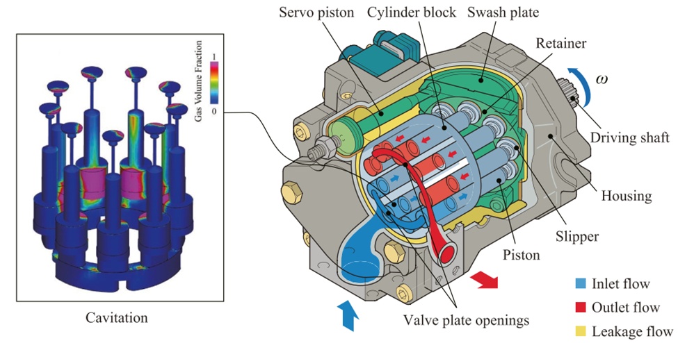
Figure 1. Construction of a swash-plate type axial piston pump
The working fluid inside the active pumping mechanisms experiences two simultaneous modes of motion: linear translation within the cylinder bores and rotational movement alongside the spinning cylinder block. The translational stroke creates a localized vacuum within the displacement chambers during the intake phase, while the rotational motion induces localized zones of low pressure near the axis of rotation [37, 38]. As a consequence, cavitation phenomena are highly prone to developing within the displacement chambers throughout the suction phase (Figure 1), particularly when the axial piston pump is driven at elevated rotational velocities or experiences reduced inlet pressures. This problematic cavitation results in a reduction of the discharge flow rate and generates elevated vibration levels across the pump housing.
The application of the Grad-CAM visualization method to boost the identification precision of cavitation within axial piston pumps is depicted in Figure 2. The unstructured vibration readings are partitioned into training and testing sets using a 4:1 ratio. Utilizing the short-time Fourier transform (STFT), the raw vibration signals within the training dataset are converted into 2D spectrogram images to facilitate the training of the CNN framework. Subsequently, class activation heatmaps are computed via Grad-CAM to establish a mask matrix that isolates the class-discriminative zones in each spectrogram image. The original spectrogram images are then multiplied pixel-by-pixel by this mask matrix to yield modified images, which are subsequently employed to retrain the CNN framework. To emulate the noisy vibration signatures encountered in actual industrial deployments, white Gaussian noise is superimposed onto the testing dataset [39]. Mirroring the preprocessing of the training dataset, these noisy testing samples are likewise transformed into spectrogram images and updated using the identical mask matrix. Ultimately, the trained CNN model processes these refined spectrogram images to identify the specific cavitation states under noisy environmental conditions.
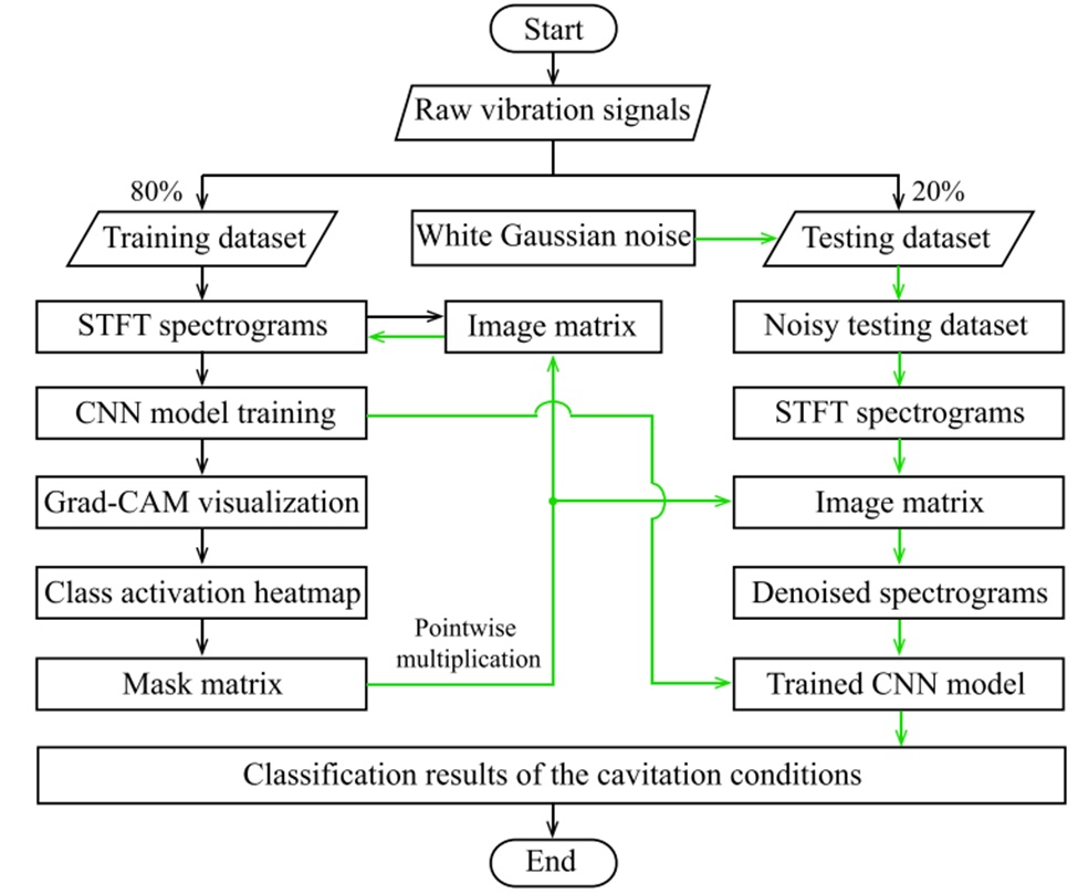
Figure 2. Flowchart of the cavitation recognition procedure
The 2D CNN model implemented in this study requires image-based inputs. The STFT represents a standard and straightforward signal processing technique capable of converting 1D time-series signals into 2D spectrogram images. The raw vibration signals are segmented into sequential data blocks containing uniform sampling points, which are subsequently mapped into spectrogram images via the STFT. The foundational principle of the STFT is illustrated in Figure 3, where a moving window function truncates the continuous data stream into windowed intervals for Fourier transformation. For a recorded vibration signal x(τ), its continuous STFT transformation at a given time instant t is expressed as [40]:
 (1)
where w ∗(t) denotes the complex conjugate of the window function w(t). Digital computation requires a discretized variant of the STFT, which is formulated as:
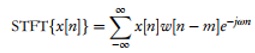 (2)
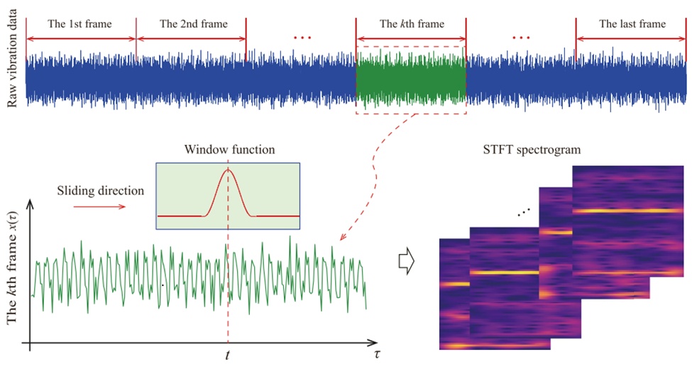
Figure 3. Schematic of STFT of vibration signal
A Hanning window is chosen for the STFT operation, and its discrete formulation is given by:
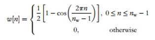 (3)
where the window length M is set to 128 in this study.
The STFT spectrogram is defined as the squared magnitude of the short-time spectral amplitude, which effectively maps the power distribution of the vibration signal across the joint time-frequency plane:
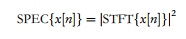 (4)
The CNN framework deployed in this research is displayed in Figure 4, representing a modified variant of the classical LeNet-5 architecture introduced by LeCun et al. [41]. The network architecture primarily comprises an input layer, convolutional layers, max-pooling layers, and fully-connected layers. The spectrogram images, sized at 128 × 128 pixels, are introduced at the input layer and subsequently routed through the convolutional and pooling layers to enable automatic feature map extraction.
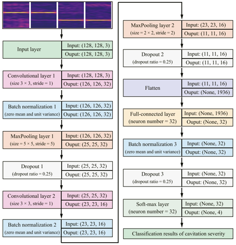
Figure 4. Architecture of LeNet-5-like network
A convolutional layer applies an array of filters to extract distinct feature maps from either the initial input images or the feature maps generated by the preceding layer. The adjustable weights of each filter are shared globally as the filters slide over the input image or feature map to capture salient patterns. The resulting output feature map can be defined as [42]:
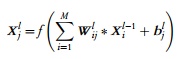 (5)
where is the i-th input feature map at layer l-1, is the j-th output feature map at layer l, represents the filter weight connecting and , is the j-th bias vector, M indicates the total set of input feature maps, and f (⋅) signifies a non-linear activation function. In this research, the rectified linear unit (ReLU), defined as f(x) = max(0, x), is chosen as the activation function.
Batch normalization is designed to establish a normal distribution by scaling the mean and variance of the activation function outputs. It enhances network stability and accelerates convergence by mitigating the "internal covariate shift" of layer activations during training. Furthermore, batch normalization renders network optimization less sensitive to the selection of hyperparameters [43] and decreases dependency on traditional regularization methods [44]. This process encompasses two primary operations: (a) data normalization across each distinct dimension, and (b) scaling and shifting modifications applied to the normalized data [20].
The pooling layer is utilized to downsample the feature maps generated by the preceding convolutional layer. Max-pooling and average-pooling represent two standard pooling strategies, which isolate the maximum and mean values within a windowed block, respectively. In this work, a max-pooling operation with a window height of H and width of W is implemented at the pooling layer:
 (6)
where represents the element located at pixel (m, n) within the feature map of layer l, and represents the element at pixel (i, j) in the feature map of layer l-1.
The dropout layer serves as a widespread regularization technique used to suppress overfitting risks in deep neural networks [45]. The core concept of the dropout strategy involves randomly and temporarily deactivating a subset of hidden units along with their respective connections during the training phase. These excluded units do not participate in specific forward and backward iterative steps. A dropout rate of 0.25 implies that one-quarter of the network nodes are disabled during training. Conversely, the dropout mechanism is turned off during the testing phase, and the layer output values are adjusted down proportionally by the dropout rate.
Following the two pairs of convolutional and pooling layers, the input image is ultimately unrolled into a flat 1936 × 1 feature vector. The initial fully-connected layer incorporates 32 hidden neurons alongside a ReLU activation function to construct a 32 × 1 feature vector. The subsequent fully-connected layer integrates 4 hidden neurons and utilizes a soft-max activation function to compute the likelihood of each distinct class:
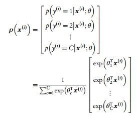 (7)
where θ = [ , , …,] represent the optimization parameters, signifies the i-th input instance, while c and C denote the c-th category and the total number of target classes, respectively. This probability distribution is normalized via the summation term 1 /(), ensuring that the collective probabilities across all classes equal unity. The soft-max classifier minimizes the following cross-entropy loss function:
 (8)
where N specifies the total count of training samples, and the indicator function 1{⋅} outputs 1 if = c and 0 if ≠ c. The training phase tunes the weight and bias parameters by minimizing this loss function via gradient descent. The CNN model configuration deployed in this study utilizes the RMSprop optimizer [46].
The developed image processing architecture leveraging Grad-CAM is illustrated in Figure 5, which aims to minimize embedded background noise and amplify feature saliency within the spectrogram images. The Grad-CAM framework utilizes the gradients of a specific target class flowing into the final convolutional layer to visualize the class-discriminative localization mapping across the input image space [47]. This visual interpretation renders the internal mechanics of the CNN model transparent and assists in identifying which precise fields dictate the image recognition process. As shown in Figure 5, the backpropagation gradient of the c-th target category relative to the k-th feature map is computed . The global weight of the k-th feature map is subsequently acquired by mapping the gradient calculation across every pixel coordinate of the feature map and averaging these values across both its width and height dimensions:
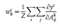 (9)
where the scalar indicates the individual contribution of the k-th feature map toward the target class c, represents the raw score computed for the c-th target category prior to the application of the softmax activation function, and denotes the pixel element at position (i, j) within the k-th feature map containing a total spatial dimension of Z pixels.
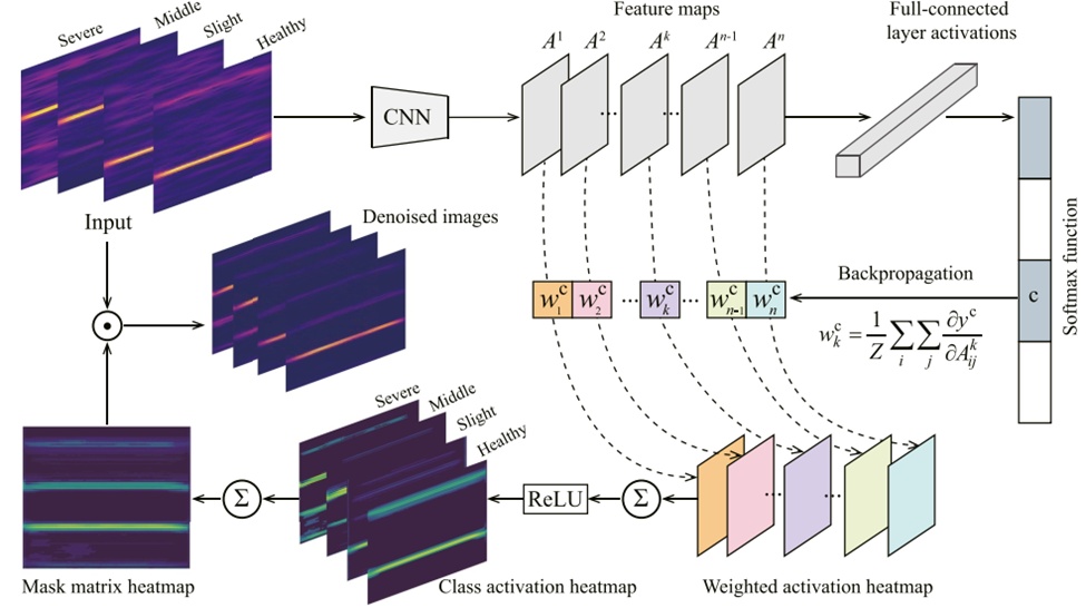
Figure 5. An overview of Grad-CAM-based image processing method
The ReLU activation function processes a weighted linear combination of all feature maps to construct the finalized class activation heatmap:
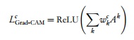 (10)
where signifies the specific class activation heatmap corresponding to the c-th target category. The inclusion of the ReLU operation in Eq. 10 serves to isolate and highlight positive pixel values while suppressing negative pixel values across the feature maps, given that the diagnostic framework is strictly concerned with features that exert a positive influence on the designated class. In general, positive and negative pixel elements within the feature maps denote the target class of interest and alternative classes, respectively. By employing the ReLU function, the localization maps are prevented from highlighting extraneous classes instead of the intended category, which would otherwise degrade spatial localization accuracy [47].
The class activation heatmaps across all specified cavitation states are acquired via an identical procedure. These maps systematically record the vital class-discriminative fields in the spectrogram images for each independent cavitation state. The individual class activation heatmaps from every cavitation condition are converted into discrete image matrices, and their algebraic summation generates a unified mask matrix :
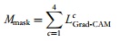 (11)
At this stage, the compiled mask matrix embodies comprehensive diagnostic data spanning all cavitation states. The yellow regions highlighted within the mask matrix heatmap denote the most critical areas required for classification. This mask matrix serves to preprocess the spectrogram images derived from the noise-corrupted vibration signals, mitigating entrained noise components and elevating feature representation prior to network deployment. Specifically, the image matrix I of each raw spectrogram image is multiplied by the mask matrix in an element-wise fashion to yield a refined image matrix :
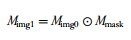 (12)
where the mathematical symbol ⊙ signifies the point-wise (Hadamard) matrix multiplication operator.
The experimental validation procedures were conducted utilizing a 1.3 \text{ cm}^3/\text{r} axial piston pump. Figure 6 displays the layout of the hydraulic network along with the physical test pump. The experimental pump assembly was driven by a variable-frequency electric motor. An oil reservoir delivered hydraulic fluid to the test pump when the primary ball valve was opened. The fluid pressure and operating temperature at the pump inlet manifold were regulated using an independent control station. The fluid pressure was adjustable across a range from 0 to 0.3\text{ MPa}, while the fluid temperature was held stable at 90^\circ\text{C}. The operating discharge pressure of the pump was governed by a system relief valve. A suite of instrumentation was integrated to track the operational state of the test pump. A speed/torque transducer recorded both the pump rotational velocity and the input mechanical torque. Two pressure transducers monitored the continuous fluid pressure at the pump inlet and outlet ports. Dual flow meters measured the structural internal leakage and external discharge flow rates within the case drain and main discharge lines, respectively. An accelerometer captured raw structural vibration datasets at the pump end cover.
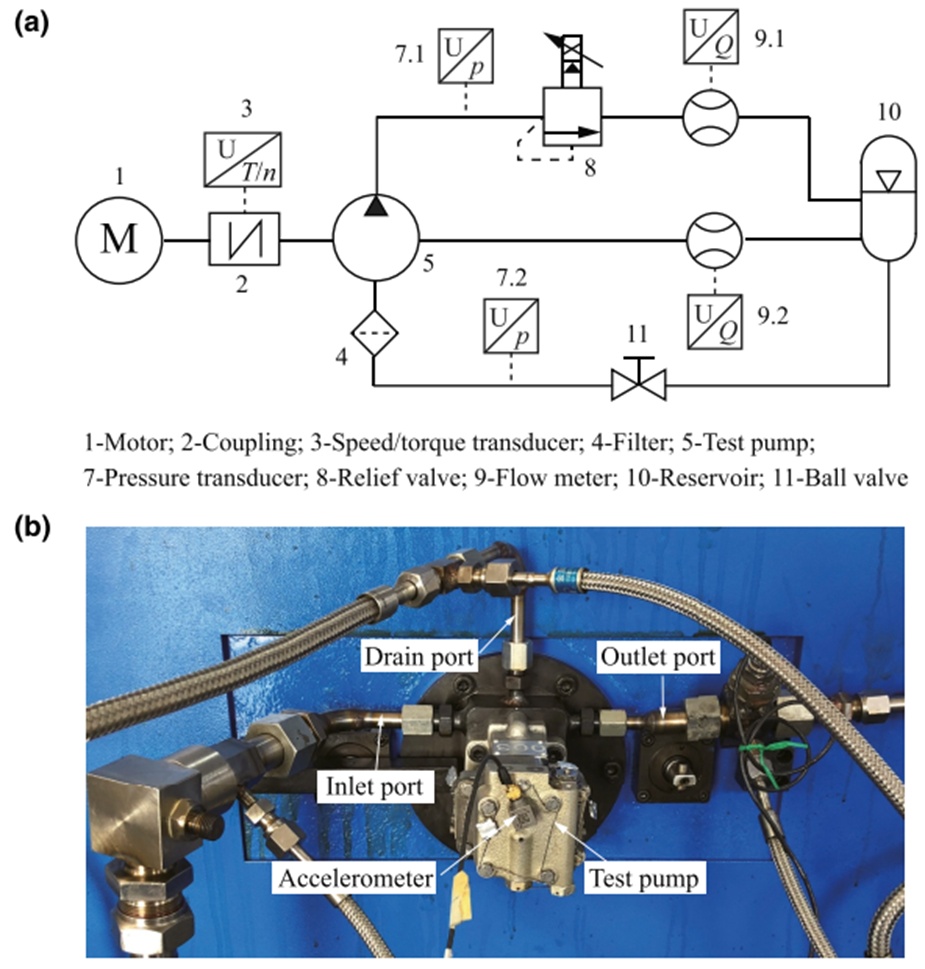
Figure 6. (a) schematic of hydraulic system; (b) test pump [4] (Reprinted with permission from Springer Nature copyright 2021)
The pump inlet pressure was adjusted to induce a range of cavitation conditions while the test pump was operated under a constant discharge pressure of 21 MPa and a rotational velocity of 10,000\text r/min, as detailed in Table 1. The inlet pressure was initiated at 0.3 MPa and incrementally decreased until active cavitation advanced within the pump casing. It should be noted that the test pump exhibited a minor volumetric loss even when running under non-cavitating conditions at an inlet pressure of 0.3 MPa. This nominal volumetric deficiency stemmed from fluid compression losses caused by oil compressibility and the high pressure gradient between the suction and discharge ports of the pump. Direct visual monitoring of cavitation formation was restricted due to the opaque metallic structure of the pump housing. Consequently, the volumetric loss ratio was selected as the indicator metric for the cavitation states, as higher levels of cavitation intensity correlate with elevated volumetric losses [8, 9]. The accelerometer recorded the high-speed vibration signatures at a fixed sampling frequency of 10,240 Hz. Figure 7 provides a comparison of the raw time-domain vibration signatures across the different cavitation states, illustrating that the vibration profiles exhibit highly similar waveforms except under the severe cavitation operating state.
Table 1. Four different cavitation conditions for the test pump
Parameter | Condition 1 | Condition 2 | Condition 3 | Condition 4 |
Inlet pressure (MPa) | 0.25 | 0.15 | 0.10 | 0 |
Ratio of volumetric losses | 1.0% | 2.0% | 8.0% | 76.0% |
Cavitation severity | Healthy | Slight | Moderate | Severe |
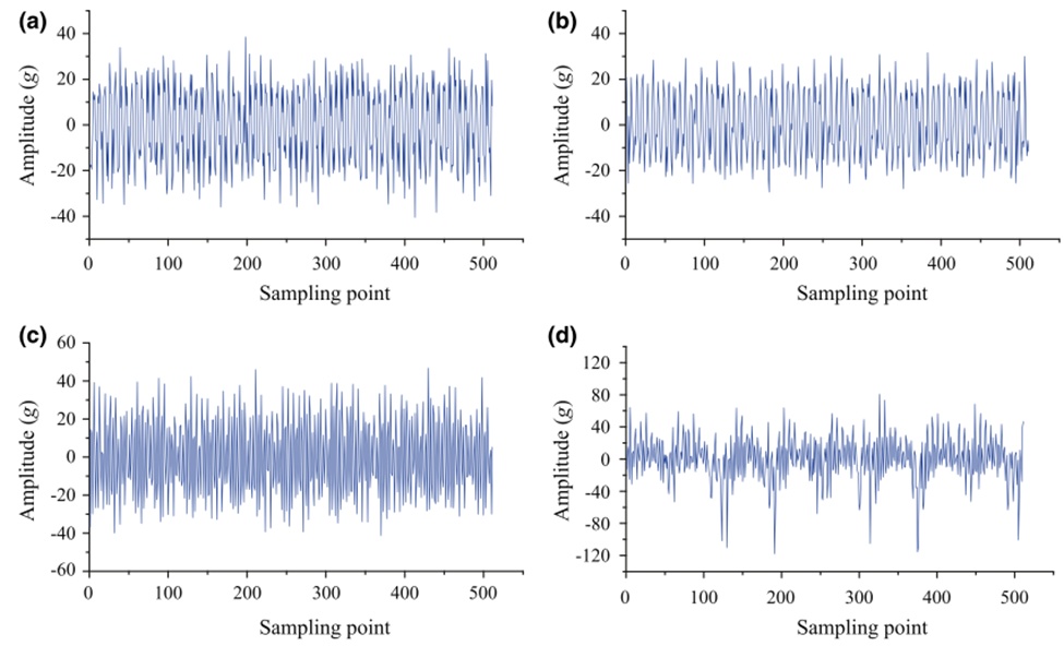
Figure 7. Vibration signals for different cavitation conditions: (a) healthy; (b) mild; (c) medium; (d) severe
Examples of the STFT spectrograms computed for all four cavitation states are displayed in Figure 8. The spectral energy of the recorded vibration signature is concentrated heavily around discrete frequencies of 1500, 3000, and 4500\text{ Hz}. Physically, the 1500\text{ Hz} component matches the fundamental piston passing frequency defined by the expression 60, where indicates the total piston count and n represents the rotational velocity. Consequently, the frequencies located at 3000 and 4500 Hz correspond directly to the second-order and third-order harmonic components, respectively. The spectrogram profiles for the four cavitation states display distinct variations in energy distribution, particularly within the frequency spectrum. Specifically, the severe cavitation condition exhibits a noticeably more dispersed energy spread across the spectrogram image compared to the alternate states. The peak spectral density of the spectrogram shifts to the second-order harmonic frequency under both the severe and medium cavitation conditions, whereas it remains aligned with the fundamental frequency for the healthy and mild cavitation states. Furthermore, the secondary peak power concentration is visible at the third-order harmonic frequency under healthy operation, yet this feature is not distinctly resolved under the mild cavitation state.
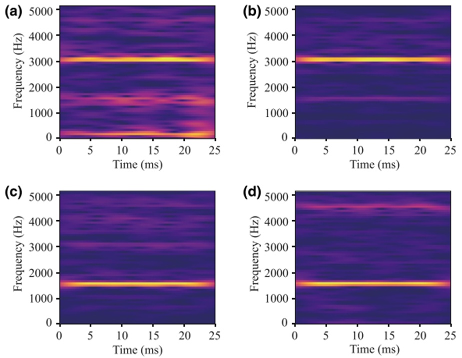
Figure 8. Spectrogram images for different cavitation conditions: (a) severe; (b) medium; (c) mild; (d) healthy
The compiled spectrogram images display unique energy distribution profiles across the various cavitation states. As a result, the baseline CNN framework successfully categorizes the four cavitation conditions, achieving an accuracy rating of 1.0 across both the training and testing datasets. Utilizing the trained CNN model and the Grad-CAM visualization pipeline, the distinct class activation heatmaps for each cavitation state are generated, as shown in Figure 9. The yellow zones highlighted within each class activation heatmap denote high activation scores for the corresponding target category. Crucially, the primary class-discriminative regions align closely with the fundamental frequency zone and its associated higher-order harmonic components within the spectrogram images. A cross-comparison of these class activation heatmaps (Figures 9a–9d) reveals that every unique cavitation state possesses exclusive class-discriminative zones within the spectrogram space. Figure 9e presents a composite heatmap constructed by summing the class activation heatmaps across all evaluated cavitation conditions. This aggregated heatmap successfully preserves the complete array of class-discriminative fields necessary for identifying all cavitation states.
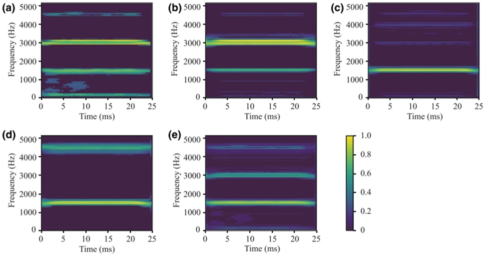
Figure 9. Class activation heatmaps over the spectrogram images for different cavitation conditions: (a) severe; (b) medium; (c) mild; (d) healthy; (e) summation of four cavitation conditions
Under practical operating conditions, background noise heavily corrupts raw vibration data, a phenomenon typically simulated using white Gaussian noise [39]. Figure 10 presents representative examples of spectrograms derived from these noisy signals at a signal-to-noise ratio (SNR) of 4 dB. In comparison to the clean baselines displayed in Figure 8, the images in Figure 10 exhibit pervasive noise distribution across the entire time-frequency domain, which introduces significant complications for accurate cavitation identification.
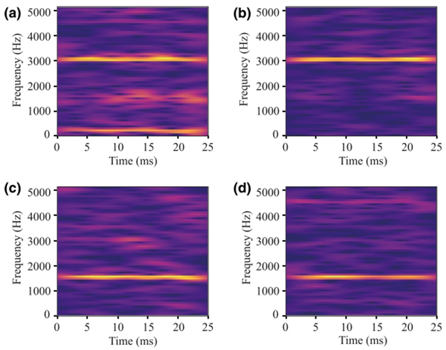
Figure 10. Spectrogram images for different cavitation conditions at a SNR of 4 dB: (a) severe; (b) medium; (c) mild; (d) healthy
The spectrograms resulting from the application of the Grad-CAM visualization method are illustrated in Figure 11. A comparative analysis between Figures 10 and 11 reveals that the Grad-CAM approach successfully isolates and removes the majority of the background noise while maintaining the integrity of the core time-frequency features representing cavitation. By filtering out irrelevant regions, the processed spectrograms appear substantially clearer, thereby strengthening the feature representation tied to cavitation behavior. Fundamentally, the mask matrix—which is established via class activation heatmaps (Figure 9)—serves to catalog empirical data regarding the class-discriminative zones that the CNN model identifies within the spectrogram.
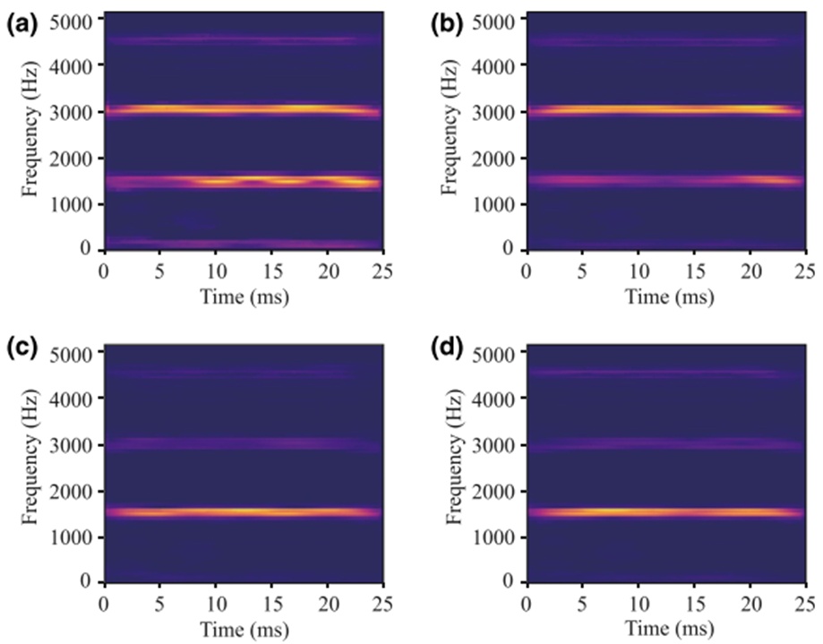
Figure 11. Processed spectrograms by the Grad-CAM for different cavitation conditions at a SNR of 4 dB: (a) severe; (b) medium; (c) mild; (d) healthy
Figure 12 evaluates the classification performance of the identical CNN architecture, comparing its accuracy with and without the integration of Grad-CAM across multiple SNR levels. As predicted, the Grad-CAM visualization tool markedly enhances the capacity of the CNN to diagnose cavitation states within high-noise environments. To illustrate, at an SNR of 4 dB, Grad-CAM elevates the detection accuracy from 0.50 to 0.89, and it boosts the rate from 0.80 to 0.92 when operating at an SNR of 6 dB.
Conversely, the performance benefits yielded by Grad-CAM become less pronounced as the SNR increases. At higher levels, such as SNRs of 8 and 10 dB, the integration of Grad-CAM actually causes marginal declines in accuracy by 0.03 and 0.04, respectively. This minor degradation is likely caused by slight structural distortions introduced into the spectrograms by the Grad-CAM mask matrix, which can precipitate image misclassification, as evidenced in Figures 9 and 11.
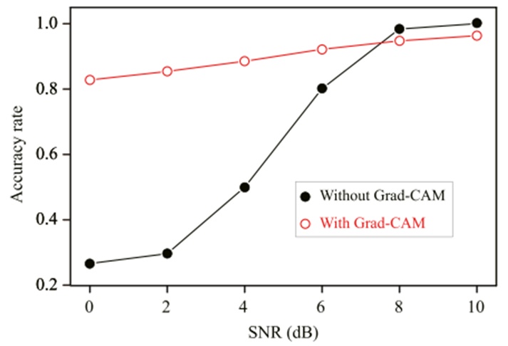
Figure 12. Comparison of diagnostic accuracy rate with and without Grad-CAM
Figure 13 provides a detailed breakdown of the confusion matrices for the diagnostic outputs generated under both testing conditions. The individual components within these matrices clarify precisely how Grad-CAM alters the classification tendencies of the CNN model. As indicated in Figure 13a, all operational states—apart from severe cavitation—undergo extensive misclassification when subjected to a low SNR of 4 dB. In contrast, Figure 13b demonstrates that the classification accuracy for these three specific categories improves substantially following the Grad-CAM image processing step. Furthermore, a comparison of Figures 13c and 13d shows that while Grad-CAM improves medium cavitation recognition by 0.06, it simultaneously diminishes the accuracy for healthy and severe states by 0.15 and 0.06, respectively. This specific trade-off explains the minor drop in the overall classification success rate observed at high SNRs in Figure 12.
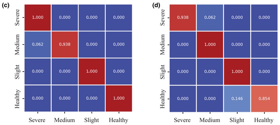
Figure 13. Confusion matrix (a) without Grad-CAM at a SNR of 4 dB; (b) with Grad-CAM at a SNR of 4 dB; (c) without Grad-CAM at a SNR of 8 dB; (d) with Grad-CAM at a SNR of 8 dB
From an industrial standpoint, detecting cavitation at its onset is a matter of high priority for executing preventive maintenance on axial piston pumps. Consequently, the automated diagnostic system must be capable of reliably spotting cavitation the moment it develops. This places a premium on achieving the maximum possible detection rate for the slight cavitation condition. Figure 14 contrasts the slight cavitation recognition rates of the CNN model with and without the aid of Grad-CAM. Because of heavy noise contamination within the spectrograms, the baseline CNN model performs poorly and yields unacceptable detection rates at low SNRs. However, once the CNN framework is coupled with Grad-CAM, the identification accuracy for slight cavitation reaches a perfect score of 1.0. For instance, as the SNR drops from 6 down to 0 dB, the tracking accuracy exhibits an improvement ranging from 0.06 to 1.0.
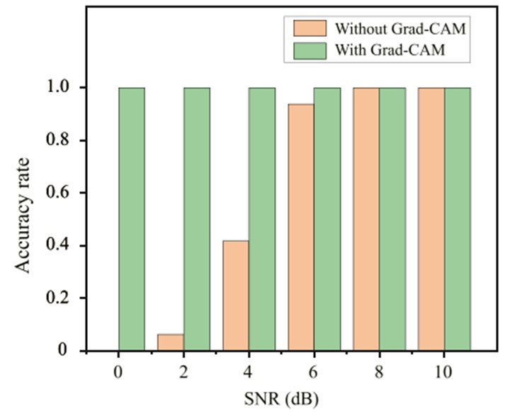
Figure 14. Comparison of diagnostic accuracy rate with and without Grad-CAM for the slight cavitation
Deploying vibration-based CNN models to detect early-stage cavitation in axial piston pumps presents a major challenge when operating in high-noise environments. This study addresses this issue by pairing the Grad-CAM visualization technique with a CNN framework to achieve dependable cavitation tracking. The trained CNN utilizes Grad-CAM to construct a customized mask matrix, which retains critical spatial data regarding the class-discriminative regions of the spectrogram for each distinct fault condition. In a deployment scenario, spectrograms generated from raw vibration inputs are pre-filtered by this mask matrix prior to being processed by the CNN network. The viability of this methodology was verified using an experimental axial piston pump subjected to four separate cavitation severities. The empirical data demonstrate that Grad-CAM drastically improves the CNN's classification accuracy in noisy settings; specifically, the collective accuracy across all fault states rises by 78% at an SNR of 4 dB and by 15% at an SNR of 6 dB. Most notably, the Grad-CAM-integrated CNN successfully identifies slight cavitation across a wide SNR spectrum spanning from 0 to 10 dB. This outcome underscores the combination of CNN and Grad-CAM as a highly viable approach for the early-stage diagnosis of pump cavitation amid heavy background noise.
The strategy introduced in this study operates under the assumption that the class activation heatmaps for all cavitation conditions contribute uniformly to the formulation of the final mask matrix. The diagnostic precision of the CNN framework could be optimized further by factoring in a weighted contribution scheme for these heatmaps. Additionally, within hydraulic networks, pressure data are often much simpler to acquire than vibration signals. Accordingly, future research directions will focus on expanding this diagnostic framework to incorporate the discharge pressure data of axial piston pumps.
This work was supported by the National Key R&D Program of China (2018YFB1702503), the Open Foundation of the State Key Laboratory of Fluid Power and Mechatronic Systems (GZKF-202108), the Open Foundation of the Guangdong Provincial Key Laboratory of Electronic Information Products Reliability Technology, the China National Postdoctoral Program for Innovative Talents (BX20200210), and the China Postdoctoral Science Foundation (2019M660086).
None
None
None
Open Access The author(s) retain copyright. This article is licensed under the Creative Commons Attribution-NonCommercial-ShareAlike 4.0 International License. It may be shared and adapted for non-commercial purposes with appropriate attribution, an indication of changes, and distribution of adaptations under the same license. Third-party material may be subject to separate terms identified in its credit line. View the license at https://creativecommons.org/licenses/by-nc-sa/4.0/.
 Transparent Intelligence Publishing