The critical nature of explainable artificial intelligence and machine learning (XAI/XML) is gaining widespread recognition. This field focuses on uncovering how input variables influence automated choices, identifying systemic algorithmic bias, and detecting vulnerability to anomalies in data. Much of the existing literature centers on creating post hoc explanations tailored for opaque, black box architectures. These secondary techniques introduce novel vulnerabilities to error without correcting the fundamental flaws of the core model. Conversely, the development of inherently transparent systems receives far less attention. This paper introduces an inherently interpretable strategy rooted in the principles of ensemble learning, designated as the League of Experts (LoE) framework. We construct the initial theoretical foundations and subsequently derive a flexible, modular meta-algorithm. Although our presentation focuses primarily on classification tasks, the LoE framework adapts identically to regression scenarios. For classification specifically, we deploy traditional decision trees to form classifier ensembles as a concrete implementation. This paradigm simplifies the extraction of human-comprehensible decision rules for the underlying classification task, yielding an independent rule-induction system called RuleLoE. Beyond evaluating 12 KEEL classification datasets, we validate the LoE framework using two benchmarks from highly critical domains—healthcare and finance—to demonstrate its utility. The predictive capability of LoE matches contemporary state-of-the-art classification algorithms regarding both accuracy and rule coverage. Furthermore, LoE outputs a highly transparent group of decision rules featuring customizable complexity to map out the target classification problem. LoE provides a dependable approach for handling classification and regression problems. Its predictive precision is highly suited for environments where discovering root causal mechanisms is the primary objective, rather than merely maximizing predictive or classification performance.
Machine learning (ML) has integrated into numerous daily applications and modern technologies, underlying progress in self-driving vehicles [1], medical diagnostics [2], and policing [3]. Legal frameworks regulating automated algorithmic determinations—such as “the right for explanation[s]” [4]—alongside other statutory considerations [5] highlight the vital need for broad transparency [6] in ML-centric systems, particularly regarding black box models. Black box systems maximize predictive metrics by compounding structural complexity to a degree that prevents human interpretation.
Current research endeavors attempt to counter this lack of transparency by layering on external systems that translate internal logic into human-readable data through added tiers of complexity (post hoc methods). However, these secondary layers function merely as rough approximations of the true decision-making pipeline and run the risk of being unfaithful to the core model [7]. Consequently, interest in explainable artificial intelligence and machine learning (XAI/XML) is expanding rapidly [8-11]. While various deployment sectors reflect the rising prominence of XAI and XML [12-14], the inherent trade-offs between accuracy and interpretability remain central to current scientific inquiry [15, 16].
This study presents the League of Experts (LoE), an original and transparent machine learning model and meta-algorithm built upon the concepts of ensemble learning [17] (p. 605). LoE operates as a specialized variant of dynamic classifier selection (DCS) frameworks [18]. Crucially, whereas conventional DCS implementations typically generate a redundant pool of classifiers using static routines like bagging or boosting [19], LoE evolves its ensemble directly during the selection and assignment phases. To our knowledge, this paradigm has not yet been investigated within the DCS literature [18].
LoE serves as an architectural blueprint that facilitates modifications tailored to maximize comprehensibility. It allows developers to create user interfaces that let human operators interact directly with the model and its subcomponents. Although this paper does not delve into specific interface configurations, it highlights potential avenues for interaction where LoE permits humans to manually tune both the selection routines and the individual ensemble units. In this manner, LoE enables users to interactively investigate the balance between model accuracy and cognitive complexity.
In this paper, we demonstrate and benchmark LoE using two distinct datasets. We focus specifically on regulating the degree of structural complexity needed to clarify the learned model instances. In addition, we present a concrete architectural configuration to implement LoE, enabling its conversion into a virtually equivalent rule set learner. To minimize structural complexity while simultaneously sharpening the approximation of the base LoE model, we further investigate methods to modify the training protocol.
In this section, we formulate the League of Experts (LoE) algorithm, detailing its design motivations regarding transparency and accuracy. To anchor this discussion, we outline the background context and taxonomy of historical and modern strategies explored within XAI and XML. T
Computing innovations have driven the use of increasingly powerful but structurally convoluted models known as black box models [20-24]. For example, feed-forward artificial neural networks (ANNs) applied to image classification tasks often contain roughly 5 to 155 \times 10^6 optimizeable parameters while performing up to 8 \times 10^{10} individual mathematical calculations for a single forward pass [25]. Because an ANN is structured as a directed graph of operations, it is technically feasible to trace every computation sequentially. In practice, however, such vast structural complexity cannot be meaningfully processed by human cognition.
Even alternative popular models that utilize significantly fewer parameters, such as support vector machines (SVMs) [26] or ensemble architectures like boosting (i.e., AdaBoost [27]) and random forests [28], defy simple interpretation. These systems are poorly suited for applications that demand a clear understanding of the decision-making logic. In ensemble learning, this limitation holds true even if the individual ensemble components are inherently interpretable, such as decision trees [29]. This problem persists because the decision boundary of the collective ensemble remains highly intricate, since the final output is generated by aggregating predictions across all participating members.
By contrast, glass box models [22, 30, 31], alternatively known as white box models, feature transparent internal operations that allow users to derive explicit explanations regarding their decision boundaries. This category includes decision trees [17] (p. 305), (logistic) regression [17] (p. 119), and instance-based neighborhood algorithms that explain predictions through the proximity of related data points, such as k-nearest neighbors (k-NN) [32].
However, introducing excessive complexity compromises practical intelligibility—such as deep decision trees with too many levels or Bayesian networks featuring excessive dependencies [33]. Crucially, this limitation stems from the cognitive boundaries of human users rather than from the mathematical mechanics of the decision-making process itself.
An illustrative instance of glass box structures is decision rules, which present analytical insight to users via intuitive logical configurations. These configurations are developed either as unordered (i.e., independent) structures known as rule sets, or as ordered sequences designated as rule lists. The latter are considerably more difficult to interpret [34] because the validity of any single rule relies on the negation of all preceding entries (meaning prior rules must fail to apply).
Decision trees can be converted into rule sets by translating each individual path from the root to a leaf into a distinct rule. For instance, the logical structure illustrated in Figure 1 corresponds to the following formulation: if (\text{sex is female} \wedge \text{age} > 40 \wedge \text{weight} > 80) \vee (\text{sex is female} \wedge \text{age} \le 40), predict low-risk group; otherwise, predict high-risk group. In contrast to decision trees, most rule induction frameworks do not generate rule sets characterized by exhaustive coverage and mutually exclusive sample space partitioning—meaning that incoming queries may satisfy either multiple rules or no rules at all. The dilemma of multiple matching rules is resolved by establishing a definitive execution order, whereas the absence of matching rules is handled by introducing a catch-all fallback rule. Both design challenges must be resolved when adapting the LoE framework into an independent rule learner
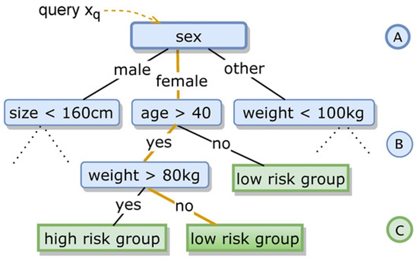
Figure 1. (Partial) decision tree example with (A–C) being the root, inner nodes, and leaves, respectively. An example query with corresponding trace is highlighted in orange.
Rule learning architectures, such as CN2 [35], RIPPER [36], Bayesian rule sets [37], Boolean decision rules via column generation (BRCG) [38], and interpretable decision sets [34], extract logical statements by directly maximizing an objective function. This optimization frequently utilizes integer programming to satisfy targeted metrics such as classification performance, coverage, or structural simplicity. Identifying the mathematically optimal solution is often computationally intractable due to the exponential growth of potential logical clauses, which reduces the task to the NP-complete set cover problem.
Within the XAI domain, the term “explanation” signifies human-comprehensible data evaluated from a local or global perspective, serving to clarify either (i) the underlying mechanism that produces an output for a specific query (such as a classification assignment) or (ii) the operational state of the entire model architecture. Local explanations can yield deceptive insights regarding the global behavior of a system, given that query-specific characteristics often do not generalize to the broader global context, i.e., across arbitrary inputs.
Post hoc explainers represent a widely used paradigm. These frameworks introduce supplementary diagnostic tools and visual interfaces designed to clarify the decision logic of a previously optimized model. Post hoc strategies are classified as either (i) model-agnostic (fully independent of the underlying algorithm class), such as LIME [39], Anchors [40], Shapley values [41], or graphical techniques like partial dependence plots (PDPs) and individual conditional expectation plots (ICE) [42]; or (ii) model-specific, which include decision-tree-tailored SHAP modifications (TreeSHAP) [43] or specialized neural network interpretability tools [44].
However, post hoc strategies exhibit notable limitations: (i) the integration of external diagnostic layers compounds the complexity of machine learning pipelines, and (ii) users must place trust in both the accuracy of the underlying machine learning model and the validity of the explanation framework itself. Either component can be erroneous, flawed, or valid only within specific unrecorded bounds. Crucially, human operators cannot easily detect these failures. Transparent glass box models bypass the need for post hoc interventions entirely, a characteristic shared more broadly by globally simulatable models that are sufficiently compact to be comprehended by a user within a reasonable timeframe [45].
Simulatable models encompass compact decision trees, restricted rule sets [46], (generalized) linear models containing a limited number of coefficients (achieved through regularization methods, e.g., Lasso), or instance-based estimators utilizing easily interpretable features (e.g., k-NN [32]). Furthermore, the features characterizing the underlying data instances must be intrinsically understandable. Models that conform to these rigorous constraints are highly restricted, often exhibiting lower predictive performance and constrained generalization capabilities [47]. Notably, the precise definition of what constitutes a simulatable model remains somewhat subjective, as it is bounded by the cognitive capacity of individual users.
Decision trees [48] directly reveal their internal logic via an intuitive graphical architecture (Figure 1). They typically isolate and evaluate only a small subset of highly informative variables or features [49], which minimizes cognitive demand on the observer. This graphical framework allows human users to closely scrutinize the nuances of a specific inference path, while also enabling the exploration of counterfactual scenarios—i.e., modifying an attribute value to observe how the downstream decision pathway alters. This capacity allows for rigorous auditing of both the fairness and the contextual relevance of the model's outputs.
Surrogate (or proxy) frameworks [50] seek to illuminate the inner workings of a complex black box model 𝑓(·) by replicating its predictive output profile across a dataset ℒ using a simpler, inherently interpretable glass box model 𝑓𝑔(·) [42] (for instance, employing a shallow decision tree to mimic a deep ANN). This mapping function 𝑓𝑐∼𝑓𝑔 can be designed to hold globally (a global surrogate) across the entire dataset ℒ, or locally (a local surrogate) within a specific subregion of ℒ. As an example, the LIME technique [40] functions as a local surrogate model.
In general, it remains difficult to verify whether the proxy model 𝑓𝑔 captures the exact causal relationships leveraged by the primary system 𝑓𝑐. A variety of structurally distinct surrogates might achieve identical approximation accuracy, a phenomenon explained by the Rashomon effect [51], which describes scenarios where multiple conflicting explanations yield identical predictive outcomes. This issue is less problematic when substituting the complex architecture with a highly precise global surrogate. For local surrogates, however, these discrepancies compound significantly, particularly if users inadvertently extrapolate global decision logic from localized explanations. While these structural vulnerabilities cannot be completely eliminated, they can be controlled and minimized by strategically guiding the training workflow.
Ensemble learning strategies [52, 53] optimize a collection of multiple base models to solve classification or regression objectives, combining their outputs via distinct aggregation or fusion mechanisms. The LoE framework aligns directly with this operational paradigm. More specifically, it represents a dynamic selection (DS) methodology [18], which diverges from static approaches (such as AdaBoost [27] and random forests [28]) by refraining from querying the entire pool of models to construct a final prediction. Instead, it utilizes an independent selection routine to isolate specific ensemble subsets for each individual input query.
The core philosophy of DS is to dynamically identify a specialized subset of models that possess high localized expertise for a given query submitted to the system. This is achieved by utilizing a filter routine that evaluates which ensemble constituents are best suited to predict a given input. This filtering routine is frequently designated as a selection or assignment function. DS methodologies are broadly classified as either dynamic classifier selection (DCS) or dynamic ensemble selection (DES) frameworks. While DCS techniques isolate exactly one model from the available pool when evaluating an incoming query, DES approaches can select a multi-model sub-ensemble. LoE is formally classified as a DCS method, as it isolates exactly one base model per query to maximize structural explainability.
To implement the League of Experts as a classification system, we modify a specific instance of ensemble learning where individual ensemble components are mapped to designated regions of the feature space. More precisely, we present an algorithmic approach that dynamically constructs a partition of the feature space to allocate a distinct, specialized ensemble component—termed the expert—to each respective subregion of the partition. Because this partitioning segments the feature space into mutually exclusive subsets, each expert undergoes training on a distinct portion of the training dataset. This process introduces diversity into the learning mechanism, implying that individual experts achieve high performance specifically within their allocated regions, but not necessarily across the entirety of the feature space. Given that individual experts do not need to capture the global characteristics of the feature space, their internal complexity can be restricted without compromising overall system performance.
The terminology for this ensemble of experts is derived from the manner in which it executes inference. Following the training of an LoE classifier, the inference phase operates via a two-stage procedure: (i) a given query x_q is directed to the appropriate expert g, and (ii) the resulting query prediction g(x_q) is computed by the designated expert (as illustrated in Figure 2). This framework mirrors cooperative human problem-solving, where multiple specialists operate within distinct domains, and a supervisor delegates assignments to the most qualified authority. As an analogy, consider a query as a patient visiting a general practitioner (acting as the coordinator) for an initial assessment. In this scenario, the coordinator routes the patient to the specialized medical professional.
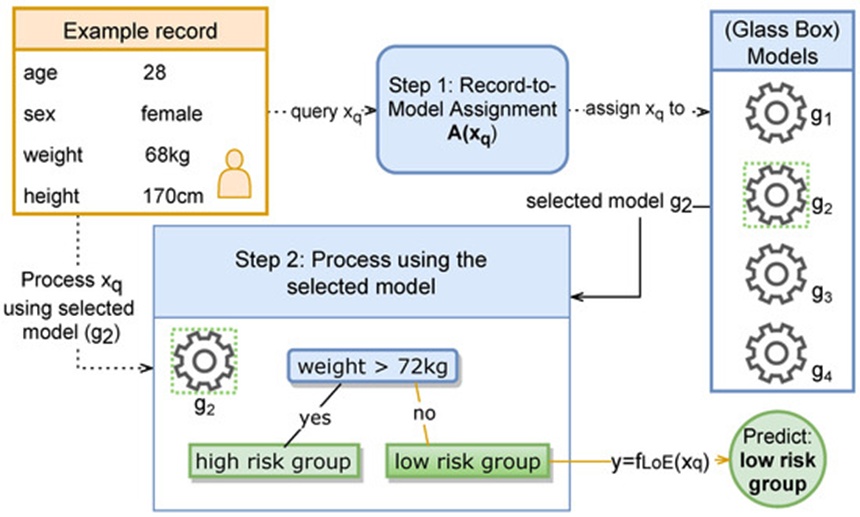
Figure 2. LoE’s two-step decision process: (i) expert assignment to query (here, g_2, a one-level decision tree) and (ii) query prediction by the assigned expert (here, prediction low-risk group). Here, experts are illustrated as gear wheels.
The subsequent subsections detail our formalizations and model architecture, our framework for generating interpretability, the minimization of explanatory complexity, the evaluation of LoE’s computational runtime complexity, and the rule-based learning variant of LoE, denoted as RuleLoE .
Let us examine a standard supervised learning scenario centered on a labeled dataset ℒ⊆𝒳×𝒞. Within this framework, each labeled instance (𝑥,y)∈ℒ is drawn from a probability distribution and comprises m real-valued features within a domain 𝒳⊆ℝ𝑚, alongside a categorical (or, for regression tasks, continuous) target label belonging to a set 𝒞 (where continuous targets satisfy 𝒞⊆ℝ𝑙). It should be noted that categorical features are permissible, provided they undergo one-hot encoding. For any given instance (𝑥,y)∈ℒ,, the objective is to maximize the conditional probability of the target variable Y given the feature vector X utilizing the model 𝑃(𝑌=𝑦|𝑋=𝑥)=𝑔𝑠(𝑥,𝑦), where 𝑔𝑠:𝒳×𝒞→[0,1] represents a probabilistic (soft) classifier chosen from a family 𝒢𝑠.
The corresponding deterministic (hard) classifier derived from this formulation is expressed as:
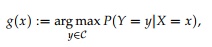 (1)
where 𝑔:𝒳→𝒞. Let 𝒢 denote the family of hard classifiers derived from 𝒢 . When addressing regression tasks instead of classification, the model targets the conditional expectation of the output Y given the input X rather than the conditional probability. Specifically, the underlying regression formulation is expressed as (ϒ|𝑋=𝑥)=𝑔(𝑥).
The mapping defined by the following function:
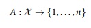
is designated as an assignment function of order n (|𝐴|=𝑛). Every assignment function A establishes a partition 𝒳= such that ∩ =∅ for 𝑘≠𝑙 across the feature space 𝒳 of rank n via the following relation:
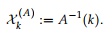 (2)
By allocating a single classifier (𝑔𝑘) to each distinct subregion () of the partition, we generate an n-tuple 𝒢∗ in 𝒢𝑛 (derived from ∈). The ordered pair (𝒢∗, A) constitutes an LoE of order n determined by A. The subregion is referred to as the territory of the corresponding expert 𝑔𝑘.
An LoE establishes a singular composite classifier via the mapping:

which typically does not belong to the original family 𝒢. The space of all valid assignment functions 𝒜 (or equivalently, the space of all corresponding geometric partitions 𝒜part) along with the classifiers 𝒢 defines the domain of all potential LoE classifiers, represented by 𝔾. It is worth noting here that the LoE framework shares conceptual similarities with DCS algorithms , where the assignment function serves the purpose of the selection mechanism. Moving forward, because any assignment function uniquely corresponds to the partition it constructs, we treat assignment functions and their corresponding partitions interchangeably.
The accuracy of an LoE classifier is evaluated using a utility metric 𝑝:𝒞×𝒞→ℝ. A standard implementation is the Kronecker delta function:
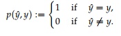 (3)
For continuous targets (regression operations), the utility metric is generally derived from a distance calculation between and y, such as the negative mean-squared error.
An optimal LoE classifier maximizes the expected utility across the joint input and output space 𝒳×𝒞; that is, it satisfies the following optimization problem:
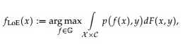 (4)
where F(x,y) represents the joint probability distribution governing inputs X and outputs Y.
The maximization problem defined in (2) is resolved via a two-tiered process: (i) for every individual assignment function 𝐴∈𝒜 (or its corresponding partition), an optimal expert collective = is determined, and (ii) these localized optimal configurations (,) are subsequently maximized across the entire space of assignment functions 𝐴∈𝒜 (or all valid partitions). This procedure yields the globally optimal LoE classifier (, A′), expressed as:
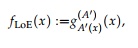 (5)
where
 (6)
and
 (7)
It is important to emphasize that an optimal LoE classifier is not guaranteed to be unique. Furthermore, computing such a classifier exactly is practically impossible, because the true underlying distribution F(x,y) is unknown and the space of potential partitions is combinatorially exhaustive. In real-world applications, an empirically pseudo-optimal LoE is resolved by substituting F(x,y) with the empirical distribution function (x,y) derived from the observed training dataset ℒ. This yields the empirical optimization formulation:
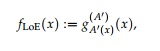 (8a)
where
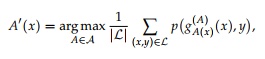 (8b)
and for each A\in\mathcal{A}
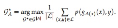 (8c)
Nonetheless, solving this empirical optimization remains computationally intractable. Generally, the spaces containing the tuples 𝒢∗ ∈ 𝒢|𝐴| (6b) and the assignment functions 𝐴∈𝒜 (6a) are uncountably infinite. However, a heuristic approximation can be achieved for restricted families of assignment functions. We introduce an algorithmic framework that produces an estimated LoE (, A∗) whose performance closely approximates that of the true optimal model.
The collection of assignment functions 𝒜 of order n is confined to the specific class of functions parameterized by n pairwise distinct anchor points 𝜃1,…, 𝜃𝑛∈ℝ𝑚 according to the following relation:

where 𝑑(·,·) represents a specified metric over 𝒳. Without incorporating the minimization operation, A would be ill-defined for instances where (𝑥,)=𝑑(𝑥,𝜃𝑙) given 𝑘≠𝑙. Consequently, we establish the following condition:
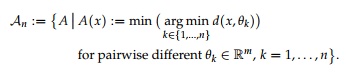 (9)
Within this framework, 𝒜𝑛 is contingent upon the selected metric d. It is recommended to choose a metric that accounts for the scale and variability of the input attributes. In this study, we utilize the weighted 𝐿1 metric (𝑥,)=|𝑥𝑖−𝑦𝑖|/𝜎𝑖, where 𝜎𝑖 denotes the empirical standard deviation corresponding to the i-th feature. In practical applications, 𝜍𝑖 is substituted by its corresponding estimate computed from the labeled dataset ℒ. An alternative approach would involve utilizing the Mahalanobis distance.
Because a bijective relationship exists between the assignment function A and an n-tuple of anchor points (\theta_1,\dots, \theta_n) for every A\in\mathcal{A}_n, these two representations are treated interchangeably. Within an LoE classifier architecture, anchor points denote the central locations of the domains governed by each expert, which is why they are designated as such.
An assignment function A segments not only the continuous feature space 𝒳 but also the discrete labeled dataset ℒ. Specifically,
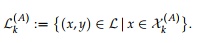 (10)
We approximate the optimization problem formulated in (6) for the class of assignment functions 𝒜𝑛 by utilizing the heuristic optimization routine diagrammed in Figure 3. This procedure initializes with n starting anchor points 𝜃1,…, 𝜃𝑛 and their corresponding assignment function A. Following this, equation (6b) is approximated with respect to the current assignment function A by optimization of a single classifier 𝑔𝑘∈𝒢 using the corresponding subset of the partitioned labeled dataset ℒ. This training yields an ensemble , thereby establishing an LoE configuration ( , A) that is "quasi-optimal for A". Next, the anchor points 𝜃𝑘 undergo an adjustment phase. We translate the central coordinates of the experts' domains, substituting 𝜃𝑘 via the following update rule:
 (11)
where 𝜂 represents the operational step size of the update. During this phase, the performance of each individual expert is quantified across the entirety of the training dataset ℒ. The domain centers 𝜃𝑘 are systematically shifted toward regions where the specific expert 𝑔𝑘 demonstrates high accuracy as quantified by the performance metric ((·),·). These adjusted anchor locations establish a modified assignment function A' along with a new partition of the underlying feature space, for which a subsequent LoE configuration is trained. This iterative step is repeated, often using systematically decaying step sizes. Ultimately, the specific LoE model that achieves the highest global performance metric is selected, which is designated as the "quasi-optimal LoE". The programmatic logic of this approach is formalized as pseudocode in Algorithm 1. The operational mechanics of the adaptation step are fundamentally dependent on the chosen performance metric. For the sake of simplicity, the Kronecker delta function (1) is implemented for the empirical evaluations detailed herein.
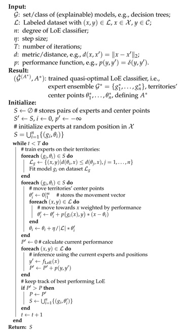
Algorithm 1. Basic League of Experts Training Procedure
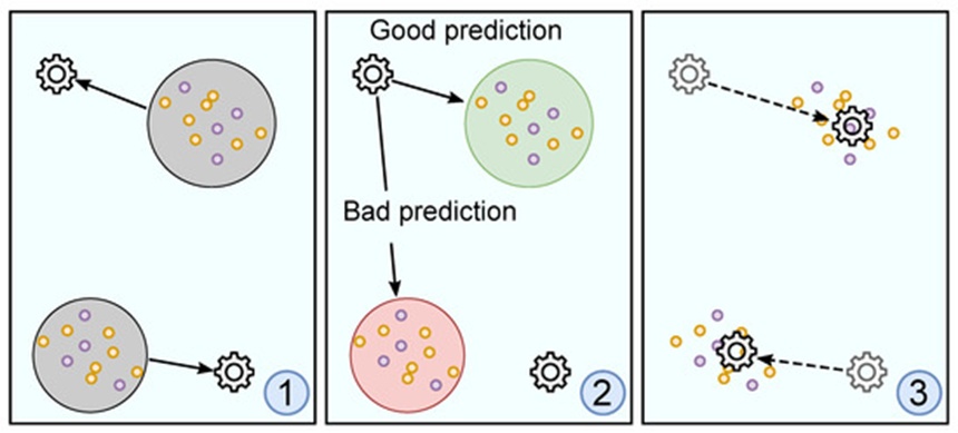
Figure 3. Training process of LoE with two experts separated into three steps: (1) data-to-model assignment (A), (2) evaluation phase, and (3) optimization phase (movement). Experts are illustrated as gear wheels. The training data are shown using purple and yellow circles, whereas each color depicts a distinct class of the learning problem. In (2), a model’s expected prediction performance on different partitions of the feature space are colored in green and red, relating to good and a bad performance, respectively.
Let (, A*) represent a quasi-optimal LoE framework where 𝐴* is defined by the final anchor positions ,…,. The resulting tuple (, A*) serves as an operational replacement for 𝑓LoE in Eq. 3. For any incoming query 𝑥𝑞, the respective distances (𝑥𝑞,) are evaluated for all 𝑘=1,…,. Subsequently, 𝑥𝑞 is routed to the corresponding closest specialized component, denoted as in Eq. 7, to calculate the final target prediction =(𝑥𝑞) (Figure 2).
In the preceding sections, we outlined a highly modular and functional machine learning architecture. When configured using glass-box models as the base experts, the framework itself is capable of optimizing an array of distinct (by virtue of being trained on mutually exclusive data partitions) and collaborative classification models (cooperating to resolve a shared target task). Although the optimized experts can independently uncover insights regarding the underlying learning task by explicitly modeling a localized component of the decision boundary, the global logic governing the assignment function remains opaque. The subsequent sections address this limitation by exploiting the structural characteristics of the architecture to extract comprehensive explanations.
Within our framework, interpretability encompasses two distinct dimensions: (i) clarifying the assignment mechanics, which explains why a given query is routed to a particular expert, and (ii) interpreting the internal logic of the experts themselves, which explains why an expert generates a particular prediction within its allocated domain. The latter aspect necessitates that the base experts are structurally transparent glass-box models—the paradigm adopted in this study—or alternatively, that post-hoc explainability frameworks are integrated. To clarify the assignment mechanics, the underlying decision boundaries generated by the assignment function A must be interpretable, a task that can be highly non-trivial. The resulting explanations must satisfy criteria of fidelity, interpretability, and exhaustiveness; these demands inherently create a trade-off, as expressed by the notion that "One Explanation Does Not Fit All [Alike]" [54].
While a wide variety of strategies exist to interpret an assignment function A (or its implicit geometric partitions), our primary objective centers on uncovering functional relationships and interactions among key features. To accomplish this, we convert the internal assignment logic into an equivalent auxiliary classification task. This surrogate task is then solved by training a glass-box model tasked with approximating the behavior of A. Although utilizing surrogate models to approximate an underlying pipeline introduces inherent fidelity risks, the LoE architecture possesses structural qualities that substantially mitigate these vulnerabilities. Most notably, a core segment of the model's predictive sequence remains completely uncompromised, because the localized experts themselves are never approximated by the surrogate system. By regulating the explicit complexity of these surrogate architectures, implementing varied modeling approaches, and integrating dimensionality reduction methods driven by a refined training pipeline, the fidelity of the surrogate approximation can be further optimized. Although a wide variety of predictive models can be adapted for this task, this investigation focuses primarily on the deployment of decision trees, as they facilitate a straightforward transformation of the trained LoE model into a structured rule-based system designated as RuleLoE.
To provide transparency for the assignment function, an interpretable glass box model is developed to serve as a surrogate for the original assignment function A. Let 𝒮 represent the family of these surrogate models, which necessitate a training dataset. The inputs fed into the assignment function consist of elements from the feature space 𝒳, whereas the corresponding labels belong to the set {1,…,|𝐴(𝒳)|}. For a specific subset 𝒳𝑠⊆𝒳 within the feature space, the graph representing the assignment function A restricted to 𝒳𝑠 is defined as follows:
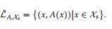 (12)
Surrogates function as assignment models themselves, though their resulting partitions generally do not belong to 𝒜. A dataset of this form can be utilized as labeled data to train a specific surrogate ℎ∈𝒮. This collection is referred to as the assignment dataset. Throughout the following sections, A represents the assignment function of a designated LoE (𝒢*, A). We structure A as a decision tree trained on the assignment dataset (meaning A is trained to map a given data point to a specific expert). The complete decision-making path for classifying a query instance 𝑥𝑞 is formulated as a concatenation of the individual decision paths from the two models A and 𝑔𝑘, where 𝑘=(𝑥𝑞), while the final prediction is expressed as =(𝑥𝑞). This procedure is illustrated in Figure 4.
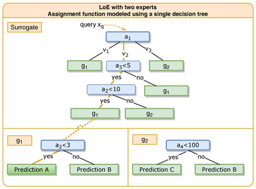
Figure 4. Exemplified LoE instance containing two experts ( and ) with A being replaced by a single decision tree (surrogate). The orange line denotes a decision path of a query (where =(,,) satisfies = ∧ < 5 ∧ < 3) through both the surrogate and one expert. At this point, it is also noted that only the expert is relevant for the query .
The capability of the surrogate to accurately replicate the baseline assignment function A (i.e., its assignment fidelity) must be assessed across a sample evaluation set ⊆ 𝒳. The degree of consistency between the surrogate h and A is quantified via (ℎ,;) , where the metric function is defined as (:𝒮×𝒜×(𝒫(𝒳)∖∅)→ℝ≥0and 𝒫 represents the power set. Higher values signify superior alignment.
If the surrogates display inadequate consistency, it implies that the model class 𝒮 might fail to capture the same underlying patterns as the components in 𝒜, or it encompasses the correct mechanisms but is overly restricted. In such scenarios, the class 𝒮 can be broadened (e.g., by loosening regularization parameters, such as permitting greater tree depth). Alternatively, the dimensionality of the input features evaluated by the surrogate can be scaled down, for example, by narrowing their feature space. Relevant projections can be determined during the LoE optimization routine.
Because the primary objective is to generate intelligible explanations for the entire operational pipeline, the clarity of the surrogate must be maintained. Consequently, surrogates must remain comprehensible. Given that the selected decision trees can grow to arbitrary levels of complexity, a metric must be established to quantify this attribute. To achieve this, we first outline the fundamental notation.
For a given decision tree t, its root node, the collection of terminating leaf nodes, and the ancestral path from a specific node v back to the root are designated as head(𝑡), leafs(𝑡), and trace(𝑡,𝑣), respectively. The decision tree routes every individual data point to a specific leaf. The trajectory for this leaf comprises the sequence of nodes spanning from the root to its arrival node. For a data subset ⊆𝒳 evaluated across the tree t, let indicate the quantity of data points within that traverse paths intersecting node v. Because the root node is included in every possible path, and exactly one unique path terminates at each individual leaf, it follows that |head(𝑡)=|| (meaning all data points initiate their trajectory at the root node).
While decision trees can regularly be mapped out through visual diagrams or translated into linear rule sets, such approaches can become unmanageable when the tree exhibits large dimensions—namely in its depth, width, or structural layout, which serve as measures of tree complexity. This perspective, however, overlooks the actual distribution of queries. Specifically, if the major proportion of queries only traverses a straightforward subtree, a structurally intricate tree can still remain practical for the vast majority of cases. The query distribution is explicitly factored in when evaluating decision tree complexity by calculating the mean trace length to the leaves for a representative sample ⊆𝒳, computed as:
 (13)
If an appropriate selection for does not emerge implicitly, it can be constructed by assuming a uniform distribution of samples across the leaves, which yields:
 (14)
Reducing the complexity of explanations
Interpretability is closely linked to the cognitive burden imposed on users. We present a strategy to minimize this cognitive load by restricting the LoE architecture to a lower-dimensional feature space. This intervention modifies the optimization process of the LoE while maintaining its predictive accuracy. This restriction likewise carries over to the assignment pipeline and is inherited by the surrogate models. Even though surrogates model intricate, nonlinear decision boundaries, most empirical datasets reside along a lower-dimensional manifold [55], which can be effectively modeled via projections.
A high-dimensional feature space containing a substantial number of attributes frequently degrades the generalization capabilities of machine learning models due to overfitting. Within the training framework of the LoE, the total number of classifiers |𝒮| scales exponentially. Consequently, multiple surrogates that fail to faithfully represent A can still display strong performance, thereby offering a justification for the assignment without reflecting the true underlying causality. This phenomenon is recognized as the Rashomon set [54].
We address the challenges of high dimensionality by mapping the full feature space onto a lower-dimensional subspace. Let 𝜋:ℝ𝑚→ℝ𝑟, specified by (𝑥)=(,…,), represent the projection of 𝑥=(,…,) onto the r target components ,…, (1≤<…<≤𝑚). The distance metric d is substituted by the (pseudo) metric (𝑥,):=(𝜋(𝑥),𝜋(𝑦)), which restricts d to the projection space established by 𝜋. Consequently, Eq. 9 is substituted by:
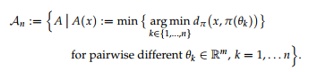 (15)
The adaptation step for the center coordinates of the expert regions is confined to this lower-dimensional projection space, leaving the remaining components unaltered; thus, Eq. 11 is adjusted to:
 (16)
where performance evaluations continue to be executed over the original, unprojected sample set ℒ. Crucially, the surrogates are trained directly within the projected feature space. This constraint limits structural complexity and curtails the Rashomon effect, thereby enhancing the fidelity of the explanations provided by the surrogate. Furthermore, user comprehension is improved because individuals are required to analyze fewer attributes simultaneously.
When decision trees are constructed using a restricted set of attributes, specific variables are more likely to reappear multiple times along a single decision path. These redundant conditions can be condensed into a single unified rule, making explanations easier to interpret. For example, if the conditions 𝚊𝚐𝚎<40 and 𝚊𝚐𝚎>30 both occur along a path, these two criteria collapse simply into 𝚊𝚐𝚎<30). In a similar manner, the combined rules (𝚊𝚐𝚎<40 and 𝚊𝚐𝚎>30) condense into the bounded expression (𝚊𝚐𝚎inrange30to40).
The formulation of a projection \pi depends directly on selecting a subset of attributes, ideally retaining those with the highest significance. For example, variables that demonstrate severe collinearity, offer minor predictive utility, or carry substantial noise can be omitted. Sophisticated implementations draw upon permutation feature importances [42] (Chapter 5.5), SHAP feature importances [42] (Chapter 5.10) built upon Shapley values [41], or direct qualitative assessments of attribute relevance provided by individual experts.
Within the context of LoE (alongside alternative DCS frameworks), the variables that exert the strongest influence on the assignment mechanism simultaneously define their own importance. Every individual expert in an LoE architecture can independently calculate attribute importance rankings, which can subsequently be aggregated into a centralized importance rating. Alternatively, these importance weights can be approximated via a surrogate model h rather than computed directly from the foundational assignment function A. This strategy requires that the designated surrogate class possesses the capability to output feature importance metrics. One potential approach involves introducing a secondary surrogate family \mathcal{S}_2 for this specific task; this family does not necessarily need to offer interpretability, but it must be capable of generating feature importance statistics. Extra trees (extremely randomized trees) [56] represent a viable option here. These models are ensembles of decision trees that utilize randomized selections of features and splitting thresholds. Because they bypass the optimization of a formal split criterion, they can be constructed rapidly while delivering robust approximations of feature importance when populated by a sufficiently large ensemble. Furthermore, they escape the structural biases induced by optimization algorithms (such as maximizing the Gini index) during the initial node split formulation.
Feature importance within the LoE framework is partially shaped during its recurrent training cycle, with importance values being extracted at each individual step. These scores can be compiled into moving averages or other time-dependent metrics that reflect long-term attribute relevance.
We formalize a specific pipeline for computing feature importances, using decision trees as the baseline architectural model. While decision trees represent an intuitive vehicle for this application, alternative models with feature-reporting capabilities can be substituted. When constructing decision trees, the ranking of attributes is intrinsically handled. The importance of any given variable is equated to its splitting utility, which is computed directly from the relative variation of a metric—such as the Gini index—during the tree-building process [57]. In the extra trees setup described previously, this metric is bypassed during the generation of the ensemble itself.
For an LoE (𝒢*,) incorporating an expert ensemble {,…,} (composed here of decision trees) evaluated on data ℒ, let signify the specific partition routed to expert (corresponding to the region where ). An importance function \phi assigns each expert the relative significance of every attribute; this constitutes a mapping from the LoE ensemble to an m-1-dimensional simplex (𝜙:𝒢*→𝒮𝑚−1) defined by 𝜙:↦((),…,()). The collective feature importance across the entire ensemble is defined as the weighted average of these relative importances across all constituent experts, formulated as:
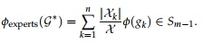 (17)
For the routing pipeline, feature importances are calculated through an independent path. Utilizing the secondary surrogate family —configured here as an extra tree ensemble containing 1000 decision trees—a surrogate model is optimized to emulate the assignment function A. An importance function analogous to 𝜙 is executed on the trained surrogate h to derive the standalone importance of each attribute. The total importance metric then averages these two components using a blending weight \alpha, as follows:
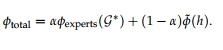 (18)
The total feature importance values are updated dynamically during each step of the LoE algorithm. Rather than utilizing these raw values directly, a temporal average is computed. The time-averaged total feature importance at iteration t, governed by a geometric decay constant \beta, is expressed as:
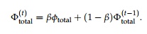 (19)
The projection \pi designed to condense the dimensionality of the feature space is established by isolating the r features that display the highest cumulative importance scores.
To map out the computational complexity of the LoE during its training phase, the analysis relies on the following parameters. First, the key operational variables dictate the overall runtime are summarized. Second, the formal training complexity of the LoE is derived.
· T = number of iterations
· 𝒢 = ensemble of experts
· ℒ = labeled dataset
· 𝐶(𝑔,(𝑥,𝑦)⊆ℒ) = training complexity for model g for data (𝑥,𝑦)
· 𝐸(𝑔,(𝑥,𝑦)⊆ℒ) = evaluation complexity for model g for data (𝑥,𝑦)
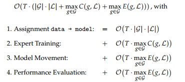 (20)
The upper bound of the iterative cycle in (20) is driven by four sequential operations that repeat across T steps: First, the current routing assignments are evaluated (1). This operation computes the distance matrix between every expert g \in \mathcal{G} and each available data point. Second, the expert optimization and spatial adjustments are performed (2). The individual experts are trained exclusively on their assigned data subsets (i.e., optimized within their local territories), a process restricted by the inherent training complexity of the specific model architectures in \mathcal{G}. Third, the optimized models are shifted along the trajectory of their highest-performing feature space positions. Finally, the updated experts execute inference tasks to determine their performance metrics (4), a phase bounded by the prediction complexity of the chosen model types.
The inference complexity of the model across a test sample 𝒳 is calculated as follows:
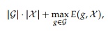 (21)
This runtime encompasses identifying the target expert (the assignment routine) and subsequently running that specific model for final prediction. Unlike traditional ensemble structures such as random forests or AdaBoost, the training duration scales with the additional multiplier T, causing the training phase to run T times slower. However, during the inference phase, only a single expert model is evaluated instead of the entire pool, avoiding the need to aggregate outputs from all ensemble members. This structure essentially demands |𝒢| distance updates plus (𝑔,(𝑥,𝑦)) for the designated or "closest" model for every x \in 𝒳. Consequently, the inference latency of an LoE model scales predictably based on the number of experts, whereas standard ensemble methods scale with the collective, aggregated complexity of all their internal models.
While LoE is not inherently designed as a rule set learner, it can be adapted into an operational equivalent known as RuleLoE by incorporating its surrogate model mechanism. For this integration, we focus primarily on decision trees serving as both experts and surrogates, though alternative rule induction algorithms can be substituted. Explicit decision rules are extracted as logical conjunctions combining two separate stages: (i) the routing pathways that dictate assignment to a specific expert (the surrogate \rightarrow expert assignment path) and (ii) the localized decision pathways within that designated expert leading down to individual leaves. The resulting decision rules are thus structured as conjunctions split into these two components.
Users can manipulate the complexity of the final rule set by adjusting parameters across both dimensions: (i) the structural complexity and approximation fidelity of the surrogate (such as enforcing a maximum depth constraint on a decision tree or applying feature space reductions) and (ii) the total volume and individual complexity of the deployed experts (contrasting a larger ensemble of simpler models against a smaller ensemble of structurally complex models). Furthermore, if a subset of experts exhibits strong global predictive power across the entire sample space, pruning the routing assignment rules can effectively boost model performance, as simplified assignment pathways are more likely to direct queries toward these highly reliable experts.
Rules generated from a singular decision tree surrogate exhibit zero overlap, meaning no two rules can be satisfied simultaneously. Although this mutual exclusivity is advantageous because it prevents prediction ambiguities, it introduces certain structural limitations. Regardless of the query routed through the pipeline, there will always be a degree of partial intersection because every query originates at the root node of the tree and consequently shares at least one initial conditional test. This constraint reduces the flexibility and structural variety of the derived rule set. However, complete rule duplication and excessive partial overlap are equally undesirable since they cause the emerging rules to become overly homogeneous.
In empirical applications, it is beneficial to exchange strict mutual exclusivity for increased rule diversity by actively minimizing partial path overlap. This is achieved by training an independent surrogate model for each available expert. The k-th surrogate learns to model the routing process relative to the k-th expert via a binary framework (a one-versus-rest strategy, or OvR). In practice, each of the k surrogates is provided with a binary-labeled dataset where a target value of 1 denotes A(x) = k (and 0 denotes all other outcomes). The surrogate learns to determine whether the k-th model should be selected to generate a prediction for a given query instance. If the condition is met, the query is assigned to the k-th expert (following its localized decision path); otherwise, no assignment occurs, and that specific expert is ignored. A visual example of this configuration utilizing two surrogates is illustrated in Figure 5. It should be noted that applying an OvR strategy within a dual-expert environment is mathematically equivalent to deploying a single surrogate, given that the target labels presented to the two models are direct inverses of each other.
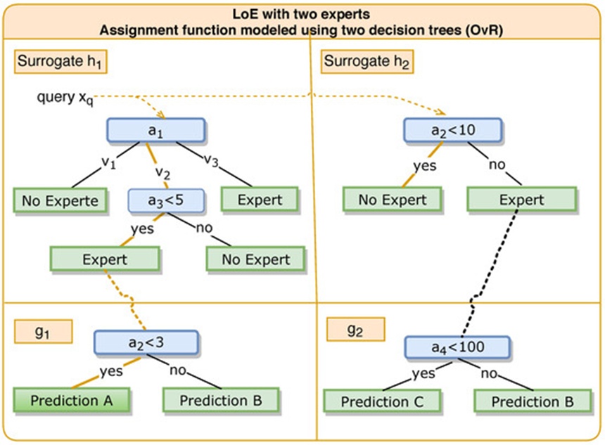
Figure 5. Exemplified LoE instance containing two experts ( and ) with A being replaced by two decision trees (surrogates). Note that this example is only illustrative as the surrogates would be inverse instances to each other in a 2-expert scenario.
Because the target labels shift for each expert when the ensemble expands beyond two models, every surrogate must be trained on a distinct data distribution. Consequently, each model uncovers unique structural patterns—especially since decision trees exhibit high sensitivity to variations in training inputs—ultimately yielding a more diverse and potentially less complex set of rules. When substituting the original assignment function with surrogate models, the underlying routing logic may not always be perfectly replicated, given that the baseline assignment function can be arbitrarily complex while the surrogate operates under strict complexity constraints or structural limitations. As a result, a given query may trigger either none or multiple expert assignments across the n surrogates.
To resolve the challenges of competing rules and unmapped queries that can occur within decision sets generated by OvR, a query resolution strategy is implemented to mimic human reasoning. When multiple rules compete for an assignment, the rule yielding the highest overall statistical performance is prioritized. Conversely, if an incoming query fails to trigger any existing rule, the closest-fitting rule is selected.
Formally, let ℒtrain represent the training dataset and denote a specific decision rule (e.g., ←𝚊𝚐𝚎>20∧𝚜𝚒𝚣𝚎<180 cm⇒ positive class). If indicates the volume of data points where rule applies, the rule's coverage is formulated as:
=|ℒ|/
The quantity of covered data points that are correctly mapped by the rule is designated as is , allowing the rule's precision to be defined as:
=
Incoming queries are mapped to rules based on the following sequential protocol:
Rank all available rules by descending precision (resolving ties by prioritizing higher coverage).
Assign the query to the covering rule that possesses the lowest rank.
If no rule directly covers , identify and return the rule that evaluates the highest proportion of its individual clauses as "true" (partial rule coverage), breaking ties by selecting the rule with superior precision.
This execution sequence, particularly step 3, is feasible only because RuleLoE operates as a multiclass rule learner. This technique cannot be applied to frameworks designed to isolate a single positive class, such as the RIPPER, CN2, or BRCG algorithms. While those alternative methods may generate smaller rule sets, they offer fewer descriptive insights into the data.
In summary, the proposed League of Experts algorithm and its structural framework provide an optimized suite of tools tailored for individuals interested in deploying, developing, and benchmark-testing explainable artificial intelligence systems. The foundational code and assets are accessible via the LoE project page and its associated repositories. The project pages for the League of Experts (LoE) ecosystem can be reached through its source repositories at https://github.com/Mereep/loe, https://github.com/Mereep/rule_loe, and https://github.com/Mereep/HDTree, accessed on 2 April 2024.
The following sections illustrate the practical application of the League of Experts algorithm and its underlying methodology using two distinct empirical datasets from the medical and financial sectors: the UCI breast cancer dataset and the HELOC dataset. Medicine and finance represent two critical domains for interpretable machine learning, as automated predictions carry significant real-world consequences. In medical environments, for instance, a patient's diagnostic path can be evaluated, modified, or clinically justified. In the financial sector, issues of systemic accountability and credit discrimination must be audited when automated systems evaluate loan applications.
Accordingly, two extensive experimental evaluations are executed and discussed below: First, LoE is implemented to analyze the structural impacts of feature space reduction. Second, LoE is converted into its RuleLoE variant, whose interpretability and predictive accuracy are systematically benchmarked against alternative rule induction systems, standard black-box architectures, and widely established ensemble methods. Following this, an in-depth structural inspection of the generated decision rules is conducted using the HELOC dataset. Additionally, a broader series of validation tests are performed across a selection of datasets from the KEEL repository under uniform baseline model settings to provide an overview of performance across varying tasks. A summary of the evaluation datasets is provided below.
Example dataset 1: UCI breast cancer The UCI breast cancer dataset (UCI breast cancer dataset, https://archive.ics.uci.edu/ml/datasets/Breast+Cancer+Wisconsin+(Diagnostic), accessed on 2 April 2024) [58] comprises 569 instances containing 32 continuous, real-valued attributes. These features describe the geometric characteristics of cell nuclei captured in digitized images of fine-needle aspirates taken from breast masses, covering metrics such as mean radius, worst perimeter, and contour smoothness. The target classification task separates instances into malignant or benign classes.
Example dataset 2: HELOC The HELOC dataset, originally released for the FICO Explainable Machine Learning Challenge (HELOC dataset, https://community.fico.com/community/xml, accessed on 2 April 2024) and utilized across multiple explainable AI studies [38, 59, 60], outlines the credit history of 10,549 individual consumers (condensed to 9,872 instances following the removal of duplicate records). The records are defined by 23 metric attributes. Loan default risk is discretized into "good" or "bad" profiles based on whether an individual incurred a payment delinquency lasting 90 days or longer within a 24-month monitoring window.
Example dataset 3: KEEL The KEEL (Knowledge Extraction based on Evolutionary Learning) dataset repository serves as a standardized testing suite designed to "aim at providing to the machine learning researchers a set of benchmarks to analyze the behavior of (...) learning methods" [61]. The KEEL ecosystem contains a wide range of datasets with diverse properties. For this validation work, a specific subset was isolated consisting of medium-scale datasets containing between 5,000 and 10,000 samples (Table 1).
Table 1. Overview of our selected subset of the KEEL dataset with sample sizes between 5000 and 10,000 samples.
Dataset | Entropy of Class Distribution | Number of Categories | Attribute Count | Number of Samples |
banana | 0.99 | 2 | 2 | 5300 |
coil2000 | 0.33 | 2 | 85 | 9822 |
marketing | 3.10 | 9 | 13 | 6876 |
mushroom | 0.96 | 2 | 98 | 5644 |
optdigits | 3.32 | 10 | 64 | 5620 |
page-blocks | 0.63 | 5 | 10 | 5472 |
phoneme | 0.87 | 2 | 5 | 5404 |
ring | 1.00 | 2 | 20 | 7400 |
satimage | 2.48 | 6 | 36 | 6435 |
texture | 3.46 | 11 | 40 | 5500 |
thyroid | 0.45 | 3 | 21 | 7200 |
twonorm | 1.00 | 2 | 20 | 7400 |
Used Software All codebases and execution frameworks were written in Python (Python project page, https://www.python.org, accessed on 2 April 2024, version 3.8). The scikit-learn library (scikit-learn project page, https://scikit-learn.org, accessed on 2 April 2024, version 0.22.2.post1) was utilized to set up and run the baseline models for random forests, gradient boosting machines, extra trees, AdaBoost, support vector classifiers (SVC), and multilayer perceptrons (MLP). The external software repositories Wittgenstein (Wittgenstein project page, https://github.com/imoscovitz/wittgenstein, accessed on 2 April 2024, version 0.1.6) and AIX360 (AI Explainability 360) [54] (AIX360 project page, https://github.com/IBM/AIX360, accessed on 2 April 2024, version 0.2.0) were deployed to implement the RIPPER and BRCG algorithms, respectively.
The total number of inputs directly impacts both the designation of the surrogate model h and how the focal points of the expert domains are modified. Here, a decision tree acts as the surrogate model. From an intuitive standpoint, minimizing the input dimensions streamlines the structural design of the surrogate, which simultaneously enhances its capacity to mimic the allocation mechanism A of the LoE.
For the empirical evaluation, the data collections are split into a 2/3 portion for model training and a 1/3 portion for model testing. The group of surrogates contains decision trees restricted to a maximum depth of 6. The architecture of the LoE is held constant as an ensemble containing n=3 experts chosen from the family 𝒢 of decision trees that possess a maximum depth of 3. On the other hand, the proportion of features saved by the projections \pi is shifted between 10% and 100% using steps of 5% (𝑟=𝑛×𝑝 with 𝑝=0.1,0.15,…,1). For every distinct value of r, the LoE undergoes training and testing across 20 separate iterations. These iterations utilize identical data partitions that are applied consistently across each step of r. The evaluation records the training and testing accuracies, the mean path distance of the surrogate decision trees h, and the allocation success metric 𝜃ass (which indicates how closely the surrogate mirrors the LoE allocation function).
Input importance is derived using Eq. 19 with assigned weights of 𝛼 =0.5 (Eq. 18) and a geometric decay rate of 𝛽 =0.3 Eq. 19). These specific parameters were not tuned for optimization. Additionally, the decision paths of the surrogates were not simplified through any consolidation techniques.
Test Results
When applied to the UCI breast cancer dataset, the LoE framework utilizing three experts demonstrates a slight tendency to overfit the training partitions. This trend is evident when comparing the training scores against the test scores (Figure 6, contrasting C and D). The training phase yields a success rate near 100%, whereas the testing phase drops closer to 94%. This divergence indicates that dropping an expert or enforcing stricter constraints on them would likely improve generalization.
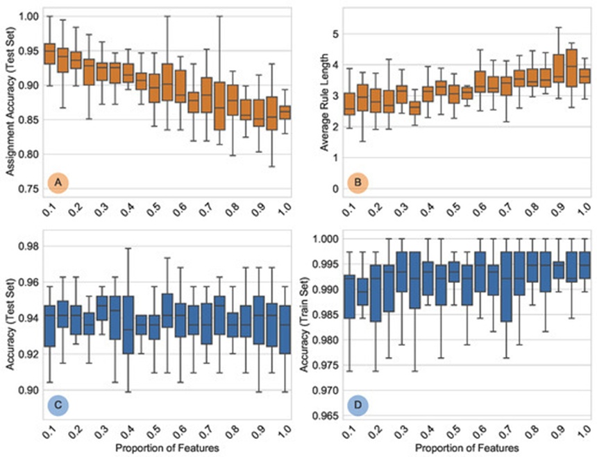
Figure 6. UCI breast cancer dataset results. Shown are paired box plots with their proportions of retained features over 20 runs for (A) assignment accuracy (p_{\text{ass}}), measured on test data, (B) average rule/path length, (C) accuracy for the test data, and (D) accuracy for the train data.
Restricting the feature space heavily impacts both the structural complexity and the overall fidelity of the surrogate model. As displayed in Figures 6A, 6B, the mean rule length (the weighted average of the path depth) shows a pronounced positive correlation with the volume of retained features (Pearson’s 𝜒2 test: 𝜒2=0.48, 𝑝<0.01). Concurrently, it displays a strong negative correlation with the allocation accuracy (the degree to which the surrogate matches 𝒜; 𝜒2=−0.62, 𝑝<0.01.
We observe parallel trends when evaluating the FICO data (Figure 7). Overall accuracy metrics are lower for both the training and testing sets, yet the underlying pattern of overfitting resembles the behavior seen with the UCI dataset (Figures 7C, 7D). However, eliminating features causes an even more dramatic shift in this scenario: the rule length shares an even stronger positive correlation with the number of attributes (𝜒2=0.57, 𝑝<0.01). Similarly, a more severe negative correlation with the allocation accuracy is present (𝜒2=−0.94, 𝑝<0.01). These powerful statistical relationships highlight how vital it is to identify the ideal target dimensionality when compressing the feature space. When more than 35% of the attributes are preserved, the mean rule length rapidly climbs toward the maximum ceiling of 6 dictated by the surrogate model family. This pattern implies that the extracted decision rules would expand in complexity if they were not artificially capped, meaning the surrogate would overfit 𝒜.
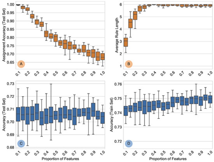
Figure 7. FICO dataset results. Shown are paired box plots with their proportions of retained features over 20 runs for (A) assignment accuracy (𝑝ass), measured on test data, (B) average rule/path length, (C) accuracy for the test data, and (D) accuracy for the train data.
The performance attributes of RuleLoE regarding (i) interpretability (mean rule length, ⌀ rules, and # rules), (ii) fidelity (rule coverage), and (iii) classification accuracy are measured against alternative rule-induction frameworks. Specifically, comparisons are made with (1) RIPPER [36] (a model that remains a state-of-the-art benchmark despite its historical background; see [46] (p. 52) and [38]), (2) Boolean decision rules via column generation (BRCG) [38], and (3) standard CART decision trees. To evaluate raw accuracy, RuleLoE is also benchmarked against two opaque black box models, SVC and MLP, which use standard parameter settings unless specified otherwise.
Given that LoE is structured as a type of ensemble learning, we also compare it against a variety of well-known alternative ensemble algorithms—specifically random forest, gradient boosting, extra trees, and AdaBoost—to offer a broader context. Because tree-based ensemble frameworks rely on concepts of ensemble capacity and maximum tree depth that match the logic of LoE, we tested two configurations for each: a default version and a matched version. The default versions use the standard hyperparameter configurations of the algorithm. The matched versions alter those default settings by locking the ensemble capacity and maximum tree depth to correspond exactly with the configurations used in LoE. The baseline ensemble setups, organized as pairs of (ensemble size / max tree depth), are configured as follows:
Random forest: 100/∞
Gradient boosting: 100/3
Extra trees: 100/∞
AdaBoost: 50/1
At this juncture, it should be clarified that standard AdaBoost only generates decision stumps, which are single-level trees with a maximum depth of one. Even though these baseline ensemble models are built from decision trees, extracting clear explanations from them is difficult because their individual outputs must be combined during the final prediction phase. Especially under default hyperparameter setups, these algorithms build massive ensembles that essentially act as uninterpretable black boxes.
The initial test configuration used an LoE ensemble composed of n=9 decision trees with a maximum depth of 1 level, alongside surrogate trees capped at a maximum depth of 2, with the feature space compressed down to r=11 attributes. Following the training process, a single expert that commanded a very small territory was manually pruned from the system.
The structural complexity of the generated rules fluctuates widely across the different models, revealing no uniform pattern. RIPPER and BRCG isolate a single target class (either positive or negative) to construct their rules, whereas LoE and CART account for both classes simultaneously, modifying both their structural complexity and performance. Consequently, RIPPER and BRCG demonstrate lower overall coverage because they map fewer data points to any given rule. In contrast, the coverage for standard decision trees (CART) reaches 100% because every possible inquiry can be traced down a valid path to a leaf node. In this evaluation, RuleLoE matches the effectiveness of the alternative frameworks, including the black box configurations. Additionally, the transparent glass box alternatives were surpassed in terms of testing accuracy (Table 2). None of the tested models sweep every evaluation category. In this scenario, there is no clear justification for choosing an uninterpretable black box model over a transparent glass box alternative.
Table 2. UCI breast cancer results. Shown are the number of rules (# rules), their average length (\varnothing rules), rule coverage, and (test/training) accuracies. Italic values for RIPPER and BRCG specify the learned positive class. Our found hyperparameters in Python notation using grid search are 𝚌𝚌𝚙_𝚊𝚕𝚙𝚑𝚊=0.01 (CART, post pruning); 𝚑𝚒𝚍𝚍𝚎𝚗_𝚕𝚊𝚢𝚎𝚛_𝚜𝚒𝚣𝚎𝚜=(200,) and 𝚖𝚊𝚡_𝚒𝚝𝚎𝚛=500 (MLP).
Method | Configuration / Target Class | Classification Accuracy (%) | Rule Coverage (%) | Average Rule Length | Total Rules |
RuleLoE | — | 94.22 / 96.28 | 96.06 / 95.21 | 1.70 | 10 |
RIPPER | malignant | 95.54 / 95.21 | 39.90 / 36.17 | 1.56 | 9 |
RIPPER | benign | 93.20 / 89.89 | 61.41 / 61.70 | 1.53 | 13 |
BRCG | malignant | 98.95 / 95.21 | 37.00 / 35.11 | 2.20 | 5 |
BRCG | benign | 99.48 / 92.02 | 61.42 / 62.77 | 2.80 | 5 |
CART | — | 97.11 / 95.74 | 100.00 / 100.00 | 3.00 | 7 |
Random Forest | default | 100.00 / 96.28 | – | – | – |
Random Forest | adjusted | 94.75 / 92.02 | – | – | – |
Gradient Boosting | default | 100.00 / 95.21 | – | – | – |
Gradient Boosting | adjusted | 94.23 / 94.15 | – | – | – |
Extra Trees | default | 100.00 / 97.87 | – | – | – |
Extra Trees | adjusted | 76.64 / 78.19 | – | – | – |
AdaBoost | default | 100.00 / 95.21 | – | – | – |
AdaBoost | adjusted | 98.95 / 96.81 | – | – | – |
SVC | — | 90.55 / 95.21 | – | – | – |
MLP | — | 94.22 / 95.21 | – | – | – |
The initial configuration consisted of an LoE ensemble composed of n=4 experts restricted to a maximum depth of 1, paired with surrogate decision trees capped at a maximum depth of 2 that preserved r=8 features. Due to an excessively high concentration of data points coupled with very poor purity (i.e., a highly skewed class distribution) at one of its terminal nodes, a single expert was manually expanded to a depth of two levels.
While RIPPER and CART extract an extensive volume of rules, they fail to deliver superior predictive accuracy (Table 3); in fact, RIPPER exhibits marginally lower performance. Furthermore, the rules generated by CART are highly intricate. Conversely, BRCG (utilizing bad as the positive class) identifies exactly one brief rule (Predict y=bad if: ExternalRiskEstimate < 73) that delivers strong predictive performance (Table 3). This aligns with expectations, as ExternalRiskEstimate serves as a highly meaningful predictor for creditworthiness; it aggregates various risk indicators to compute an overall risk score through an undisclosed functional relationship. Consequently, the straightforward classification rule produced by BRCG relies on a rigid threshold that remains opaque to external observers. In contrast, RuleLoE yields a different set of pathways, resulting in the subsequent rule set (Figure 8).
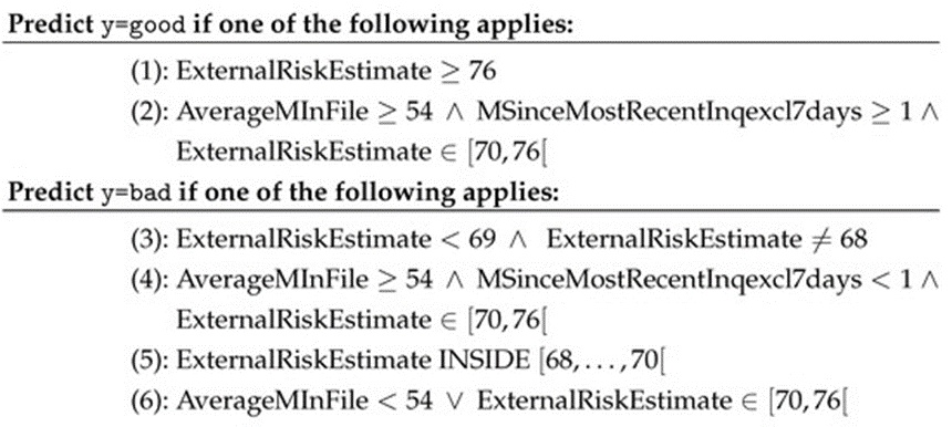
Figure 8. FICO dataset results. Shown are the obtained rules via RuleLoE.
Table 3. FICO dataset results. Shown are the number of rules (# rules), their average length (⌀ rules), rule coverage, and (test / training) accuracies. Italic values for RIPPER and BRCG specify the learned positive class. Our found hyperparameters using grid search are ccp_alpha=0.001 (CART, post pruning); hidden_layer_sizes=(8,8) (MLP).
Technique | Variant / Target Label | Prediction Accuracy (%) | Coverage of Rules (%) | Mean Rule Size | Number of Rules |
RuleLoE | — | 72.04 / 71.73 | 100.00 / 100.00 | 2.00 | 6 |
RIPPER | bad | 73.95 / 70.03 | 50.44 / 49.66 | 2.50 | 18 |
RIPPER | good | 73.95 / 71.49 | 47.05 / 47.39 | 2.40 | 25 |
BRCG | bad | 71.12 / 70.38 | 56.01 / 56.29 | 1.00 | 1 |
BRCG | good | 72.35 / 70.53 | 48.50 / 48.22 | 3.00 | 2 |
CART | — | 74.05 / 71.24 | 100.00 / 100.00 | 4.86 | 21 |
Random Forest | default | 100.00 / 72.41 | – | – | – |
Random Forest | adjusted | 100.00 / 72.41 | – | – | – |
Gradient Boosting | default | 62.25 / 62.83 | – | – | – |
Gradient Boosting | adjusted | 76.70 / 73.20 | – | – | – |
Extra Trees | default | 71.12 / 70.38 | – | – | – |
Extra Trees | adjusted | 62.49 / 62.86 | – | – | – |
AdaBoost | default | 74.89 / 72.71 | – | – | – |
AdaBoost | adjusted | 71.05 / 69.28 | – | – | – |
SVC | — | 73.20 / 72.41 | – | – | – |
MLP | — | 71.58 / 70.17 | – | – | – |
Certain pathways from this set could undergo further consolidation, such as rules (3) and (5). Nonetheless, these classification pathways inherently incorporate the same opaque metric, ExternalRiskEstimate. However, unlike the binary thresholding of BRCG, this model uncovers additional contextual information. Whenever the metric ExternalRiskEstimate fails to provide an unambiguous signal for a favorable or unfavorable credit rating (≥76 or <70, respectively), the case is treated as borderline, and the final assessment shifts to two fully transparent attributes. Specifically, applicants are designated as having a favorable credit score if their history spans a mean of more than 54 months in system records and their most recent credit inquiry occurred more than 1 month prior. Formally, a credit profile is deemed favorable if AverageMInFile≥54∧MSinceMostRecentInqexcl7days<1. In all other instances, the profile is classified as unfavorable.
These more informative decision paths produced by RuleLoE exhibit lower structural complexity than the alternative techniques, with the sole exception of BRCG configured for the positive class bad, which occasionally yields marginal performance gains (Table 2). As a consequence, opaque black box models do not generally outperform transparent glass box frameworks regarding accuracy within our tested scenarios; notably, the SVC achieves only a negligible edge over the remaining algorithms. Weighing all evaluated criteria, RuleLoE demonstrates superior overall utility compared to the alternative approaches, as it facilitates active knowledge discovery by generating straightforward, highly interpretable decision pathways that maximize explainability.
For the entire suite of evaluations involving the KEEL archive, we deployed an LoE ensemble featuring three distinct experts restricted to a maximum depth of 2. This highly constrained architecture was intentionally chosen to prioritize the extraction of compact, easily interpretable rule architectures, directly supporting the core objective of generating explanation-driven models. The underlying data were partitioned using a standard 2/3 split for training and testing stages. To establish a comparative baseline, a random forest model was evaluated under identical constraints regarding ensemble volume and maximum tree depth (Table 4).
Even without implementing dataset-specific hyperparameter tuning, the LoE achieves a thoroughly respectable level of performance. A few of our experimental trials reveal a low allocation accuracy (specifically on the marketing and texture data segments), which subsequently penalizes the downstream performance of RuleLoE. This degradation can likely be traced to an inadequate depth configuration within the corresponding allocation trees or an insufficient degree of feature reduction. The data segments corresponding to marketing, optdigits, and texture—which demonstrate suboptimal overall metrics—are characterized by a high number of distinct classes (Table 1). These multi-class landscapes cannot be adequately mapped by decision trees restricted to a depth of only two levels, naturally introducing higher misclassification rates. On average, however, both LoE and RuleLoE surpass the restricted random forest architecture in terms of predictive accuracy, highlighting the structural advantages of LoE for generating efficient, highly interpretable rule-based systems under strict architectural constraints. Consequently, future research should investigate these specific performance variations in greater depth, incorporating a broader array of baseline models.
Table 4. Test results for the KEEL dataset, comparing the accuracy of LoE, a derived RuleLoE, and a random forest classifier as pairs of train/test accuracies. Additionally, the number of rules and their average length is reported. Best average results are highlighted in bold.
Dataset | Extracted Rules (Average Length) | Assignment Precision (%) | RuleLoE Performance (%) | LoE Performance (%) | Random Forest Performance (%) |
banana | 10 (2.20) | 99.35 / 99.31 | 83.55 / 82.68 | 83.75 / 83.02 | 64.74 / 63.87 |
coil2000 | 4 (2.75) | 99.83 / 99.91 | 94.01 / 94.08 | 94.18 / 93.99 | 94.01 / 94.08 |
marketing | 1 (2.00) | 28.29 / 26.87 | 18.35 / 18.06 | 32.48 / 32.91 | 27.25 / 27.97 |
mushroom | 8 (3.62) | 99.07 / 99.52 | 98.92 / 99.41 | 99.84 / 99.89 | 90.08 / 89.43 |
optdigits | 8 (3.88) | 57.24 / 58.22 | 52.88 / 51.27 | 65.34 / 63.83 | 55.35 / 56.93 |
page-blocks | 5 (2.80) | 98.01 / 98.28 | 94.27 / 93.58 | 95.69 / 94.57 | 93.97 / 93.47 |
phoneme | 9 (3.11) | 90.08 / 89.69 | 76.69 / 76.35 | 79.53 / 79.93 | 75.58 / 76.18 |
ring | 9 (2.44) | 84.79 / 84.77 | 73.26 / 71.25 | 76.32 / 74.12 | 76.38 / 74.53 |
satimage | 10 (3.40) | 83.86 / 84.42 | 77.38 / 78.30 | 82.16 / 83.57 | 71.12 / 71.05 |
texture | 9 (3.33) | 62.61 / 63.86 | 60.22 / 59.89 | 70.91 / 70.19 | 36.28 / 35.32 |
thyroid | 5 (1.60) | 98.13 / 98.40 | 98.11 / 98.36 | 97.57 / 98.15 | 94.63 / 93.98 |
twonorm | 3 (3.00) | 75.47 / 75.23 | 74.16 / 75.39 | 94.61 / 94.27 | 80.33 / 79.81 |
Mean Across Datasets | 6.75 (2.84) | 81.39 / 81.54 | 75.15 / 74.88 | 81.03 / 80.70 | 71.64 / 71.38 |
In this study, we introduced the League of Experts (LoE) framework as a novel architectural paradigm within the fields of explainable artificial intelligence and explainable machine learning (XAI/XML). The LoE represents a unique class of ensemble learning that integrates surrogate models specifically designed to maximize model interpretability and enable seamless human-in-the-loop interaction. Working alongside this architecture is RuleLoE, a specialized rule-induction method derived from the parent ensemble. By selecting individual ensemble components—the experts—exclusively from transparent glass box models, the broader LoE framework functions inherently as a glass box system. As our experiments demonstrate, this approach maintains competitive predictive performance when evaluated against established glass box algorithms and opaque black box models alike. Crucially, feature space compression mechanisms can be natively embedded directly into the LoE training sequence, thereby reducing the structural complexity of the resulting explanations. This offers a stark contrast to conventional methodologies that must navigate through high-dimensional feature spaces without such safeguards. Moving forward, we intend to focus on hyperparameter optimization, targeting both the establishment of robust baseline defaults and the automated contextual tuning of ensemble components based on specific dataset characteristics and runtime training diagnostics.
As a result, numerous pathways for refining both LoE and RuleLoE remain to be fully investigated concerning operational usability, predictive throughput, and explanation visualization. While our current experimental validations utilized decision trees as the core building blocks for the LoE, the framework accommodates a wide variety of base learners. Incorporating alternative model classes could enable the architecture to capture distinct attribute distributions more effectively, while blending heterogeneous models might map highly intricate data distributions while fully preserving system explainability. To ensure the practical utility of these methodologies, comprehensive options for direct user interaction (such as pruning specific nodes from decision paths, establishing whitelists or blacklists for certain attributes relative to designated experts, or manually discarding individual pathways from RuleLoE) must be built into intuitive user interfaces. The development of these tools will be guided by targeted user experience studies. An interface of this caliber would ideally streamline the injection of domain-specific human expertise directly into the active machine learning pipeline. Structured user interaction has the clear potential to minimize latent algorithmic biases and enhance causal decision mining. Accordingly, this initial introduction of the LoE framework serves as a foundational benchmark for subsequent advancements.
The following abbreviations are used in this manuscript:
ANN | artificial neural network |
BRCG | Boolean decision rules via column generation |
CART | classification and regression trees algorithm |
DCS | dynamic classifier selection |
DES | dynamic ensemble selection |
DS | dynamic selection |
DSEL | split of training data used in some MCS algorithms |
ICE | individual conditional expectation plots |
k-NN | k-nearest neighbors |
LoE | League of Experts |
MCS | multiple classifier system |
ML | machine Learning |
MLP | multilayer perceptron |
OvR | one-versus-rest |
PDP | partial dependence plots |
RuleLoE | League of Experts rule set learner |
SVC | support vector classifier |
SVM | support vector machine |
TreeSHAP | decision-tree-based SHAP |
XAI | explainable artificial intelligence |
XML | explainable machine learning |
None
None
This study was carried out in the group of junior scientists “Agile Publika”, which is funded by the European Social Fund (ESF) and the Free State of Saxony, Germany. The work of Kristan Alexander Schneider was partially performed within the DFG project “SCH 1480/2-1”.
None
Open Access The author(s) retain copyright. This article is licensed under the Creative Commons Attribution-NonCommercial-ShareAlike 4.0 International License. It may be shared and adapted for non-commercial purposes with appropriate attribution, an indication of changes, and distribution of adaptations under the same license. Third-party material may be subject to separate terms identified in its credit line. View the license at https://creativecommons.org/licenses/by-nc-sa/4.0/.
 Transparent Intelligence Publishing