To overcome critical constraints regarding diagnostic accuracy and model transparency in medical imaging, this paper presents a novel framework termed the Pixel-Level Interpretability (PLI) model. The investigation primarily aims to benchmark PLI against Gradient-Weighted Class Activation Mapping (Grad-CAM) to attain superior localization correctness and highly detailed explainability. Operating on a VGG19 convolutional neural network infrastructure, the methodology incorporates three open-access COVID-19 chest X-ray datasets containing over 1000 categorized images; these underwent augmentation, normalization, and resizing steps to achieve generalizability and algorithmic stability. The experimental evaluation focused on vital performance metrics: structural similarity (SSIM), mean squared error (MSE), interpretability, computational speed, and diagnostic precision. The findings indicate that PLI drastically surpasses Grad-CAM across every evaluated metric. Specifically, PLI generated fine-grained, pixel-granular heatmaps that yielded reduced MSE, superior SSIM metrics, and expedited inference rates, demonstrating an capability to reveal minute diagnostic elements without sacrificing processing speed. Conversely, the explanations produced via Grad-CAM regularly lack the detailed resolution necessary for dependable clinical integration. By incorporating fuzzy logic to refine both numeric and visual explanations, PLI delivers transparent data that corresponds with clinical logic, thereby allowing healthcare professionals to execute decisions with greater certainty. Ultimately, this research validates PLI as a dependable framework for resolving deficiencies in AI explainability and clinical adoption. By simultaneously managing the dual demands of precision and transparency, PLI advances medical AI deployment and establishes a precedent for implementation within other high-stakes environments.
Artificial intelligence (AI), particularly deep learning frameworks like convolutional neural networks (CNNs), has reshaped the landscape of clinical diagnostics by facilitating highly accurate identification of pathologies from radiological scans. Despite demonstrating exceptional performance, these architectures frequently draw criticism for operating as "black boxes," yielding clinical predictions devoid of underlying logic. This deficit in operational clarity damages clinical confidence, presenting major roadblocks in high-stakes fields like medicine, where secure, verifiable, and transparent outcomes are mandatory for sound patient care decisions.
The expanding deployment of AI systems within clinical workflows highlights the urgent necessity for explainability, making it vital to clarify not just the final prediction but the underlying algorithmic reasoning. Contemporary options frequently rely on post hoc interpretability frameworks, including Gradient-Weighted Class Activation Mapping (Grad-CAM), Local Interpretable Model-Agnostic Explanations (LIMEs), and Shapley Additive Explanations (SHAPs). Though these approaches have broadened our insight into AI decision-making, they possess major vulnerabilities. Grad-CAM yields broad, low-resolution visual maps that fail to provide the pixel-level specificity needed to detect subtle pathological anomalies in medical scans. Similarly, while LIMEs and SHAPs offer attribute-level breakdowns, they cannot translate these findings into pixel-level precision, which restricts their utility in clinical settings that require meticulous, localized evidence. Consequently, these drawbacks slow down the successful integration of AI systems in medicine, particularly where precise localization and transparency are crucial.
To resolve these deficiencies, this research introduces the Pixel-Level Interpretability (PLI) model, a hybrid convolutional–fuzzy architecture that pairs fuzzy logic operations with CNN-derived class activation mapping. PLI elevates interpretability and diagnostic accuracy alike by supplying highly detailed, pixel-granular visual mappings of AI decisions. This design guarantees precise target localization for diagnostic features, equipping clinicians with functional data that matches their professional reasoning and encourages confidence in computer-aided diagnostics. Deviating from standard methods, PLI successfully bridges the divide between diagnostic precision and explainability, making it uniquely appropriate for medical environments where high precision and transparency are non-negotiable.
The primary goal of this research is to perform a rigorous comparison of PLI and Grad-CAM, targeting specific explainability criteria such as accuracy, coherence, selectivity, and continuity explanation. The study applies a rigorous experimental framework using three open-source COVID-19 chest radiograph repositories to confirm the system's performance relative to these targets. The anticipated outcomes intend to demonstrate PLI’s superiority over Grad-CAM regarding both clinical accuracy and interpretability, while also showcasing its processing efficiency and compatibility with practical healthcare operations.
Integrating artificial intelligence (AI) systems into diagnostic imaging has brought the necessity of explainability to the forefront as a requirement for establishing trust in clinical settings. Current approaches, such as Grad-CAM, LIMEs, and SHAPs, have advanced our comprehension but cannot generate the pixel-granular clarity mandatory for pinpoint diagnoses. This analytical review examines these existing methodologies, their implementation within medical imaging, and their operational constraints, highlighting the demand for pioneering strategies like the Pixel-Level Interpretability (PLI) model to reconcile the tension between explainability and precision in AI-assisted medicine.
The use of AI, especially deep learning tools like convolutional neural networks (CNNs), has drastically optimized accuracy and throughput in clinical diagnostics. Nevertheless, widespread adoption within hospital environments remains constrained due to deficiencies in model explainability [1]. Medical professionals demand complete transparency before trusting AI-generated outputs, particularly in high-stakes scenarios where patient lives are affected. Algorithms functioning as uninterpretable "black boxes" fail to win institutional trust, regardless of how high their diagnostic accuracy rates may be [2, 3].
Model interpretability is frequently modeled as the inverse of architectural complexity: as models grow more intricate and highly accurate, their internal transparency tends to diminish. Consequently, the tools developed within this domain are meant to clarify AI findings during clinical decision-making, allowing healthcare staff to act with greater assurance and ease [3]. Figure 1 illustrates the overarching structural relationship between algorithmic complexity, performance accuracy, and machine learning interpretability. To illustrate, rudimentary frameworks like linear models offer high interpretability but typically yield substandard accuracy. Intermediate structures, such as decision trees, achieve a moderate balance of both transparency and precision. Lastly, highly intricate frameworks like neural networks or CNNs deliver maximal accuracy alongside minimal interpretability. This classic trade-off underscores the difficulty of balancing algorithmic performance with clear transparency, especially in critical spaces like medical institutions [4].
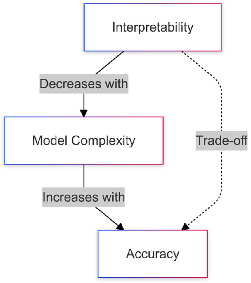
Figure 1. The relationship between model complexity, interpretability, and accuracy in AI applications in healthcare [4].
A variety of explainability frameworks have been engineered to demystify the internal mechanics of intricate AI systems. Saliency-based approaches, exemplified by Gradient-Weighted Class Activation Mapping (Grad-CAM), illuminate decisive spatial zones within an image, whereas attribute-centric frameworks like LIMEs and SHAPs isolate the significance of individual features. Additionally, rule-centric paradigms offer straightforward decision logic, and hybrid methodologies attempt to unify localized and global perspectives. In spite of their distinct advantages, these techniques frequently encounter constraints, such as a deficiency in pixel-level resolution or diminished performance on high-resolution, fine-grained tasks. This section analyzes the competencies and boundaries of these diverse strategies, highlighting their vital role in the realization of transparent and dependable AI architectures.
(1) Class Activation Mapping (CAM) and Grad-CAM: Grad-CAM is frequently deployed owing to its operational simplicity and its capacity to produce visual saliency maps that highlight the spatial regions guiding algorithmic classifications [5]. Nevertheless, the resulting explanations are structural and lack the pixel-granular detail required to detect subtle pathological variations [6].
(2) Layer-Wise Relevance Propagation (LRP): LRP establishes pixel-level importance by backpropagating attribution scores from the output layers to the initial input nodes. This strategy provides highly granular feedback but is heavily restricted by and dependent on the underlying neural network configuration [7].
(1) LIMEs (Local Interpretable Model-Agnostic Explanations): LIMEs approximate the behavior of complex systems on a localized scale using simplified surrogate models to clarify individual predictions [8]. Though highly effective for feature-level assessments, adapting this framework for pixel-granular decomposition remains constrained.
(2) SHAPs (Shapley Additive Explanations): Grounded in cooperative game theory, SHAPs compute individual feature attributions to provide mathematically rigorous global interpretability. Its deployment for pixel-level medical diagnostics continues to be underutilized [9].
The Anchors framework establishes conditional rules that are sufficient to validate specific classifications; however, this methodology is inherently more compatible with structured tabular datasets than with the pixel-level spatial analysis required for clinical radiographs [10].
MAPLEs (Model Agnostic Supervised Local Explanations): By combining localized and global explainability, MAPLEs excel at deciphering highly non-linear feature interactions, yet they lack native architectural provisions for processing image-based data structures [11].
Grad-CAM remains the dominant methodology in terms of clinical popularity due to its uncomplicated deployment and overall efficacy, securing the highest adoption metrics among current options. Systems like LIMEs and SHAPs follow closely in utilization, whereas Anchors and MAPLEs remain less widely integrated due to structural limitations in specialized domains such as clinical imaging.
Saliency-based explainability architectures within the medical imaging domain are indispensable for deciphering and visualizing how machine learning (ML) and deep learning (DL) systems formulate diagnostic outputs. These frameworks illuminate the precise topographic zones of clinical scans that exert the most profound influence on algorithmic outputs, thereby empowering radiologists and clinicians to evaluate automated findings with increased efficiency [12]. Table 1 summarizes the diverse AI-centric interpretability frameworks utilized across clinical imaging, detailing their primary characteristics, diagnostic tasks, advantages, and inherent constraints [5, 7, 13-15]. The primary categories of heatmap-based explainability frameworks routinely integrated into medical imaging workflows include the following:
Table 1. Overview of interpretability methods in medical imaging.
Method | Key Feature | Medical Imaging Applications | Advantages | Limitations |
PLI | Provides pixel-level interpretability using heatmaps | CT, MRI, ultrasound, and CT scans; helpful for diagnosing conditions with subtle anatomical changes | Offers detailed, pixel-specific insights; increases clinician trust and transparency | Performance depends on data; requires diverse datasets for generalization across imaging modalities |
Saliency Maps | Highlights pixel influence via gradients | Detection of lesions and anomalies | Easy to implement | Sensitive to variations in input data |
Class Activation Maps | Focuses on the final convolutional layer | Identifying disease-specific regions | Class-discriminative; highlights specific regions | Restricted to certain CNN architectures |
Grad-CAM | Uses gradient-weighted localization | Flexible localization of pathologies | Compatible with various CNN models | Focus on high-level features limits fine detail |
Guided Grad-CAM | Combines Grad-CAM with backpropagation | Detection of small features, such as microcalcifications | Provides fine-grained visualization | Computationally demanding |
Layer-wise Relevance Propagation (LRP) | Propagates relevance layer by layer | Analysis of histopathology images | Offers detailed, pixel-level relevance information | Complex and dependent on network architecture |
Integrated Gradients | Integrates gradients smoothly | Detection of subtle features (e.g., tissue irregularities) | Generates smooth and interpretable heatmaps | Choice of baseline can impact results |
SmoothGrad | Reduces gradient noise | Accurate localization, e.g., retinal scans | Produces clearer, less noisy heatmaps | Higher computational overhead |
Occlusion Sensitivity | Assesses effect of occluding regions | Evaluates region criticality, e.g., breast cancer | Intuitive and insightful | Computationally expensive |
PLI constructs high-resolution visual heatmaps that identify critical anatomical zones within diagnostic scans. These maps offer authentic Pixel-Level Interpretability, mapping the specific structural regions that dictate classification choices, with attribution indices spanning a range from 0.1 to 1 [6]. This allows medical practitioners to map algorithmic predictions directly to exact anatomical markers, which builds institutional trust and accelerates the integration of AI tools into clinical workflows [14]. While conventional explainability tools generally produce broad, image-wide feature attributions, the PLI framework introduces a fine-grained interpretability paradigm at the individual pixel layer. This produces a more logical explanation by calculating the explicit contribution of solitary pixels—a vital requirement in clinical settings where physicians must verify the precise pathological boundaries driving a diagnostic conclusion. Ultimately, this transparency enhances accountability in AI-assisted choices. However, the operational fidelity of the PLI framework remains heavily dependent on the diversity and baseline quality of the underlying training data. Crucially, expanding evaluation repositories to encompass a wider array of medical imaging modalities will ensure robust generalization across a diverse spectrum of real-world clinical scenarios [15].
Grad-CAM expands the utility of activation mapping to a wider variety of CNN architectures by removing the structural requirement for global average pooling. This methodology leverages the gradients of the model's target output relative to the feature tensors of the final convolutional layer to calculate pixel importance, making it possible to visually isolate the regions driving algorithmic predictions [5]. Within clinical diagnostic spaces, this technique facilitates highly flexible network designs that help refine the identification of localized pathologies, such as bone fractures on CT scans or oncological lesions in mammography [16]. Consequently, this model design displays high adaptability across diverse CNN variations and custom network architectures. Its principal benefit lies in its widespread versatility across various deep learning frameworks, enabling it to conform to diverse engineering constraints. Conversely, a major drawback stems from its complete reliance on abstract, high-level convolutional layers, which limits its diagnostic utility for intricate, fine-grained visual tasks that require highly localized, low-level spatial analysis [17].
Saliency maps identify the specific image regions that exert the greatest impact on model predictions by calculating the gradients of the output relative to the input pixels. This approach facilitates the identification of regions of interest, including lesions or anomalies within clinical scans, by highlighting the specific features driving the system's choice [18]. The primary benefit of saliency maps lies in their algorithmic simplicity and their straightforward demarcation of target zones. Conversely, the most critical constraints of these techniques include their vulnerability to noise and high sensitivity to trivial input variations, which can compromise their dependability in medical environments where precision and structural stability are vital [19].
CAMs leverage the final convolutional layer of a CNN to produce a class-specific heatmap that preserves spatial characteristics, which is subsequently employed to localize discriminative features within an image [20]. This method illuminates the specific topographic zones most relevant to a given classification category, such as the detection of tumors on MRIs or lung opacities on chest CT scans [21]. A major advantage of CAMs is their class-discriminative property, which permits exact localization for individual target categories. However, this architectural constraint typically restricts their application to CNN configurations that incorporate global average pooling immediately preceding the output layer [22].
Guided Grad-CAM functions by merging Grad-CAM with the Guided Backpropagation mechanism to supply high-resolution, pixel-level detail for enhanced explainability. This framework pairs the regional importance calculated by Grad-CAM with high-resolution visual feedback. While Grad-CAM isolates the broader macroscopic regions critical for classification, the refined output from Guided Backpropagation allows only positive gradients to propagate backward, adding structural detail to the generated insights [23]. This capability is exceptionally beneficial in medical imaging for isolating minute pathologies or microcalcifications. Its principal advantages center on fine-grained visualization, which markedly improves clarity and precision. Nonetheless, the method is computationally intensive and susceptible to noise artifacts, which may degrade its reliability in specific clinical imaging tasks [24].
LRP is an explainability method designed to backpropagate the relevance score of the final output layer step-by-step through the network layers down to the primary input pixels. The resulting LRP-based heatmaps provide a fine-grained visualization of individual pixel contributions to the final decision, distributing the total output score across the input layer. This technique has become increasingly important in medical imaging domains like histopathology due to the high complexity inherent in image interpretation [25]. The primary benefit of LRP is its capacity to deliver pixel-level relevance data, offering a granular view of model reasoning. Although it introduces greater complexity than Grad-CAM or basic saliency maps, LRP remains an interpretability tool that is heavily dependent on the specific network architecture employed [26].
Integrated gradients evaluate the path integral of gradients along a straight line from a specified baseline image to the target input image. This procedure yields a smoother heatmap by integrating gradients over multiple intermediate steps between the baseline and the input. It highlights the regions most influential to the model's classification, which is highly advantageous when analyzing subtle or diffuse visual features, such as tissue irregularities in MRI or CT scans [27]. The primary strengths of this approach are the generation of continuous, highly interpretable heatmaps and the reduction of gradient noise, resulting in clearer visualizations. However, it is highly dependent on the choice of an appropriate baseline and can be computationally expensive due to the requirement of calculating gradients across multiple steps [28].
SmoothGrad enhances the visual quality of standard saliency maps by mitigating the high-frequency noise inherent in traditional gradient-based attribution methods. This is achieved by adding random Gaussian noise to an input image across multiple iterations, generating an ensemble of perturbed images, and subsequently averaging the resulting saliency maps [29]. This process yields a cleaner, less noisy heatmap that improves overall interpretability and localization precision. This technique is highly effective in diagnostics requiring meticulous localization, such as identifying vascular abnormalities in retinal photography [30]. Although SmoothGrad offers the benefit of smoother and more readable heatmaps, it demands a higher computational budget because multiple perturbed inputs must be synthesized and processed [31].
Occlusion sensitivity mapping offers a transparent and intuitive approach for evaluating model predictions by systematically masking different spatial regions of an image and measuring the resulting effect on the model's output probability [32]. This technique has been effectively utilized within medical imaging to isolate regions of interest. For instance, in mammography, specific segments of breast tissue can be occluded to monitor variations in prediction, allowing areas linked to potential abnormalities to be identified with high clarity based on the importance assigned by the model [33]. The most compelling benefits of this strategy are its conceptual simplicity and intuitive interpretation. The primary limitations of this method include its high computational demands, as multiple forward passes are required to evaluate each masked region sequentially [34].
These diverse frameworks provide clinicians and researchers with a rich selection of methodologies to decode intricate neural networks used in medical imaging. These tools underpin the comprehension of machine learning outputs by highlighting distinct dimensions of image data, thereby closing the operational gap between deep learning models and clinical diagnostic deployment [35].
Fuzzy logic was originally introduced by Zadeh in 1965 as a mathematical framework for reasoning under uncertainty [36]. It is uniquely suited for domains such as medical imaging, where diagnostic choices must frequently be formulated based on ambiguous, vague, or imprecise data [37]. The utilization of fuzzy logic in medicine encompasses diverse areas, including automated disease diagnosis and clinical risk assessment [38]. Fuzzy systems possess the capacity to model complex, uncertain relationships that are difficult to capture using traditional Boolean logic. Within the sphere of AI interpretability, fuzzy logic has been integrated to produce more granular and comprehensible explanations from deep learning models [39]. Unlike classical logic, which operates within a strict binary true/false framework, fuzzy logic introduces continuous degrees of truth. Consequently, it allows for a more nuanced understanding of the interactions between input features and model predictions [40]. This capability is highly relevant to medical image analysis, given the subtle visual transitions that frequently separate healthy and pathological tissues [41]. Because fuzzy logic accommodates partial truths and inherent uncertainty, it serves as a powerful instrument for interpreting CNNs by treating activation maps as fuzzy sets and executing rule-based inference to derive more transparent outputs [42].
Several studies have investigated the fusion of fuzzy logic with deep learning systems to achieve enhanced explainability. For example, Fuzzy Cognitive Maps (FCMs) have been deployed to model complex clinical ecosystems, promoting transparency in decision-making by blending embedded expert knowledge with raw data patterns [43]. Similarly, Fuzzy Neural Networks (FNNs) have emerged as robust hybrid architectures that unite the optimization capabilities of neural networks with the intrinsic interpretability of fuzzy systems, as depicted in Figure 2 [44].
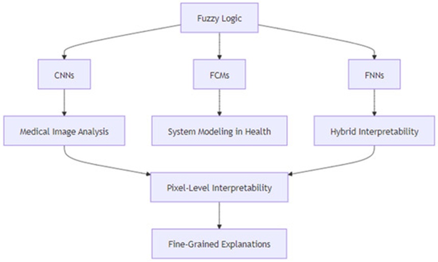
Figure 2. Framework for Fuzzy logic integration in AI-driven medical imaging images [4].
This section outlines the empirical framework for classifying chest CT scans to differentiate COVID-19-positive instances from healthy control subjects utilizing Pixel-Level Interpretability (PLI) and Gradient-Weighted Class Activation Mapping (Grad-CAM). Both interpretation techniques are built upon the VGG19 architecture, a convolutional neural network (CNN) model pretrained to ensure dependable analysis of medical images. The investigation implemented these methods to isolate infected pulmonary regions, comparing their diagnostic performances to establish which framework yields more informative and dependable observations for clinical workflows. Figure 3 illustrates the sequential phases of the comparative research pipeline: dataset preprocessing, model training, and the generation of heatmaps. The concluding stage centers on comparing the resulting heatmaps to assess the utility of both methodologies, as illustrated in Figures 6 and 7, regarding their interpretability and target localization precision. Qualitative evaluations were performed via visual examination of the heatmaps produced by the PLI and Grad-CAM systems.
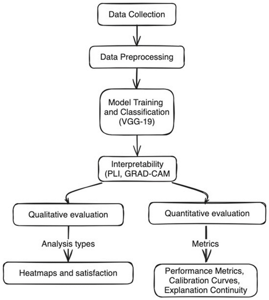
Figure 3. Workflow of the comparative methodology for diagnosing COVID-19 using chest CT scans.
Three open-access repositories of thoracic radiographs, containing more than 1000 categorized scans (classified as either normal or COVID-19-positive), were utilized and authenticated by expert radiologists. This empirical data is openly and freely available on the Harvard Dataverse repository via the link https://doi.org/10.7910/DVN/6ACUZJ (Accessed on 22 November 2024) [45].
(1) Resizing: All source images underwent dimensional adjustment to a standardized size of 224 × 224 pixels to satisfy the structural input specifications of the VGG19 framework.
(2) Normalization: Pixel intensity values were scaled to accelerate network convergence and maintain operational consistency across the input dataset.
(3) Data Augmentation: To expand data variance and augment model resilience, transformation methods including spatial rotation, mirroring, and luminance adjustments were enforced.
(4) Noise Reduction: Gaussian filtering was applied to mitigate background image noise, thereby accentuating features of diagnostic significance.
The experimental trials were executed utilizing NVIDIA Tesla V100 graphics processing units (GPUs), with TensorFlow 2.x serving as the underlying deep learning framework. Routine data execution and process automation were facilitated through specialized Python scripts.
A comparative performance assessment between PLI and Grad-CAM was carried out via paired t-tests to evaluate metrics including accuracy, precision, and recall.
Confidence bounds were computed for each diagnostic performance metric to affirm statistical significance and ensure the stability of the empirical findings.
Figure 4 details the operational flowchart of the PLI framework, which introduces a substantial progression in explainability techniques by directly overcoming the constraints of current approaches like Grad-CAM [6]. By leveraging fuzzy logic frameworks—incorporating fuzzification, rule inference, and defuzzification stages—it integrates into the system to refine explainability at a pixel-specific resolution. In contrast to Grad-CAM, which relies on high-level feature map pooling, this algorithm implements 19 trapezoidal membership functions and localized fuzzy rule bases to yield discrete insights regarding individual pixel attributions. Furthermore, the algorithm adjusts the standard Grad-CAM methodology by embedding fuzzy thresholds, ensuring that the generated visual outputs are both mathematically sound and clinically functional. Figure 5 illustrates the deployment of Grad-CAM within the VGG19 infrastructure for classifying CT scan data. It complements the mathematical developments shown in Figure 4 by mapping how these diverse strategies converge inside the organized pipeline outlined in Figure 3. Together, these illustrations map the progressive optimization of interpretability and diagnostic accuracy. A qualitative assessment of the saliency maps was performed by visually reviewing those derived from both PLI and Grad-CAM. These evaluations focused on three distinct categories: (1) Clarity: The ease with which the highlighted anatomical areas could be understood. (2) Granularity: The degree of physical detail present within the isolated zones. (3) Diagnostic Relevance: How closely the highlighted segments corresponded with verified clinical markers of pathology. The PLI maps demonstrated superior localization fidelity and enhanced visual contrast when isolating critical tissue zones compared to Grad-CAM, confirming the heightened explainability of the PLI framework. The core original insights are detailed below:
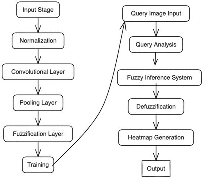
Figure 4. Workflow of PLI model [6].
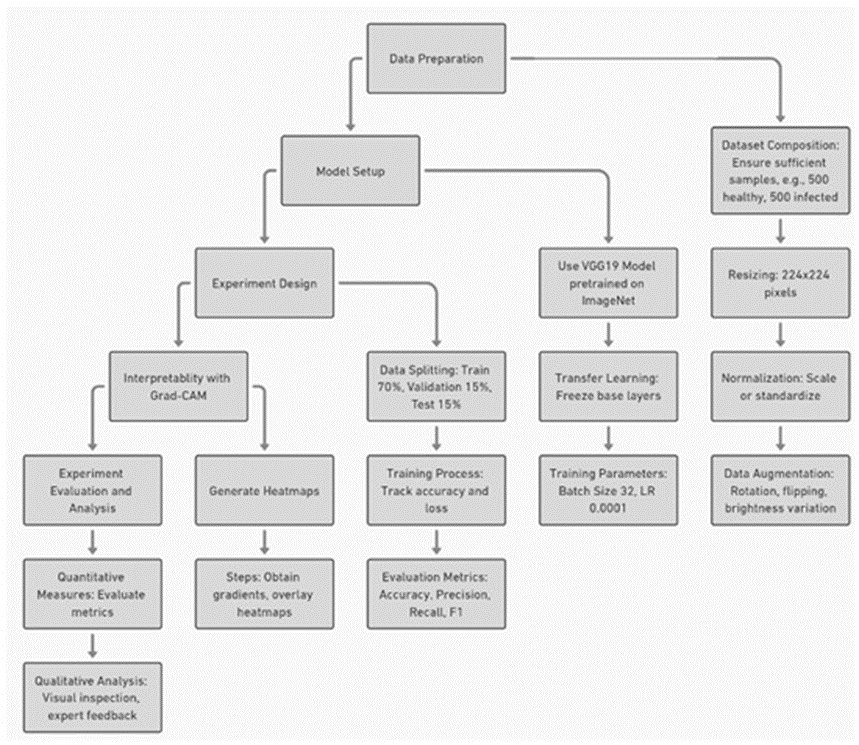
Figure 5. Workflow of COVID-19 CT scan image classification using VGG19 and Grad-CAM.
1. Fuzzy Logic Integration: This broadens the capabilities of PLI by translating CNN feature representations into fuzzy sets, facilitating highly nuanced explainability at the individual pixel layer.
2. Localized Precision: This optimizes the broad, low-resolution visual mappings generated by Grad-CAM by focusing explicitly on individual pixel contributions and their underlying clinical weight.
3. Hybrid Adaptability: This alters both PLI and Grad-CAM architectures, bridging historical gaps regarding feature resolution and real-world clinical deployment.
In brief, the algorithm categorizes any target image into three distinct classifications using 19 trapezoidal membership functions to achieve an optimal balance of precision, interpretability, and generalizability. The procedural steps are detailed sequentially below:
1. Input Stage: Individual CT scan images are ingested in either grayscale or RGB format, establishing the primary data matrix for computational evaluation.
2. Normalization: Pixel matrices are scaled to a uniform range of [0, 1], mitigating data variances stemming from heterogeneous imaging environments.
3. Convolutional Layer: Convolutional masks are applied to isolate structural features such as margins and textural variations that indicate the presence of infection markers.
4. Pooling Layer: Spatial down-sampling is executed via maximum or average pooling operations, maintaining critical feature geometry while decreasing the computational workload.
5. Fuzzification Layer: Raw pixel intensities are converted into fuzzy membership values, assigning mathematical degrees of probability (e.g., elevated or reduced) regarding pathological presence to boost clarity.
6. Training: The operational bounds of the fuzzy membership functions are determined from the pixel data, establishing thresholds that separate diseased lung structures from healthy tissue.
7. Query Image Input: An unseen evaluation CT scan is introduced, subjected to preprocessing, and evaluated against the established fuzzy thresholds.
8. Query Analysis: The pixel attributes of the query scan are benchmarked against the trained fuzzy membership intervals to compute the likelihood of pathology.
9. Fuzzy Inference System: Spatial fuzzy rules, such as "if infection likelihood is elevated, then classify pixel as infected," are executed at the individual pixel level to formulate classifications.
10. Defuzzification: The aggregated fuzzy values are transformed into explicit, discrete classifications, specifically categorizing regions as either "infected" or "healthy".
11. Heatmap Generation: A localized saliency map is constructed to visually depict high-probability or infected anatomical regions using color spectrum gradients to assist clinical assessment.
12. Output: The final product consists of the high-resolution heatmap, structured for direct application in medical diagnostic operations.
The automated classification of COVID-19 pathology within thoracic CT scans followed a structured pipeline centered on the VGG19 model architecture, matching the approach delineated by [46] and illustrated in Figure 5. This diagnostic process comprised three primary phases: data compilation, network configuration, and experimental planning.
The image repository was structured and processed using scaling, intensity normalization, and geometric data augmentation methods to maximize model stability and ensure broader generalizability.
(1) Base Model Initialization: The VGG19 architecture, initialized with weights pretrained on the ImageNet repository, was employed as the foundational feature extraction engine. Three dense, fully connected layers were integrated at the termination of the network to customize it for the binary classification objective (distinguishing COVID-19-positive scans from normal controls). These added components comprised a dense layer containing 512 nodes with ReLU activation, followed by a dropout layer (configured at a rate of 0.3) to mitigate overfitting risks, and a terminal dense layer utilizing a sigmoid activation function to output the final classification probabilities.
(2) Transfer Learning: The convolutional layers of the pretrained VGG19 model (comprising all 16 convolutional stages) were initially locked to preserve broad, low-level feature extraction competencies. Subsequently, incremental fine-tuning of the uppermost 4 convolutional layers was carried out to adapt the network to the specific binary classification task. This targeted fine-tuning process was executed using the specialized COVID-19 CT scan repository, which had been preprocessed via scaling and data augmentation methods.
(1) Data Splitting: The image repository was divided into a training subset (70%), a validation subset (15%), and an independent testing subset (15%).
(2) Batch Size Optimization: Computational runs were evaluated using batch allocations of 32, 64, and 128. A batch size of 64 was ultimately chosen to maintain an ideal balance between GPU memory constraints and training convergence stability.
(3) Learning Rate Tuning: Optimization tracks were analyzed across learning rates of 10−2, 10−3, and 10−4. A learning rate of 10−4 demonstrated the most effective compromise between optimization speed and numerical stability.
(4) Number of Epochs and Early Stopping: Model training was scheduled for a maximum duration of 50 epochs, with an early termination policy enforced if the validation loss failed to improve over 10 consecutive validation checks. The optimal model parameters were achieved at epoch 30, matching the point where the validation loss reached a stable plateau.
(5) Regularization Methods:
(a) Dropout: Dropout percentages of 0.2, 0.3, and 0.4 were evaluated, with a configuration of 0.3 producing the highest validation precision and generalization performance.
(b) L2 Regularization: An L2 regularization penalty featuring a \lambda weight of 0.001, selected via cross-validation techniques, successfully contained model overfitting and reinforced generalizability.
(6) Weight Initialization: He initialization was applied across all layers utilizing ReLU activation functions, maintaining stable output variance through successive network depths and accelerating optimization convergence.
(7) Optimizer: The Adam optimization algorithm, configured with standard hyperparameters (\beta_1 = 0.9, \beta_2 = 0.999), was selected due to its adaptive learning rate behavior and efficient performance in the presence of sparse gradients.
(8) Loss Function: Binary cross-entropy was applied as the objective loss metric, matching the requirements of the binary classification task and optimizing the probabilistic tracking between the two target classes.
The neural network underwent optimization incorporating early stopping safeguards, minimizing overfitting tendencies while maximizing predictive accuracy and field generalizability. Vital performance metrics—specifically accuracy, precision, recall, and F1-score—were rigorously verified against both the validation and independent testing datasets.
Following preprocessing, the target CT scans were routed through the fully optimized VGG19 architecture, which generated final probabilistic scores for the binary classification task (COVID-19-positive vs. normal).
Figure 5 outlines the sequential procedures required to apply Grad-CAM for explainability enhancement through the creation of activation heatmaps that visually mark the anatomical segments dictating the network's choices. The global architecture of Grad-CAM relies on a systematic progression through these individual phases [5]. Qualitative valuation was performed by visually auditing the saliency maps produced by both the PLI and Grad-CAM frameworks. These empirical reviews concentrated on the underlying clarity, feature resolution, and diagnostic utility of the isolated zones. The PLI framework yielded superior localization boundaries and heightened visual contrast when pinpointing critical pathological developments compared to Grad-CAM, verifying the optimized interpretability of the PLI model:
(1) Compute gradients: The gradients of the target classification score relative to the feature tensors of the final convolutional layer are evaluated to formulate the underlying Grad-CAM activation map.
(2) Overlay heatmap: The resulting activation map is superimposed directly onto the source CT scan, visually highlighting the localized tissue regions that drove the model's categorical classification.
This section presents a detailed assessment benchmarking the Pixel-Level Interpretability (PLI) model against the Grad-CAM framework using compiled collections of thoracic radiographs. The experimental trials assess essential dimensions, including visual interpretability, diagnostic categorization precision, computational throughput, and the spatial continuity of explanations. Through integrated quantitative and qualitative evaluations, this investigation demonstrates the capacity of the PLI framework to yield highly localized, transparent, and clinically applicable insights, highlighting its core structural benefits over standard interpretability methodologies.
This subsection explores the visual outputs generated by both the Pixel-Level Interpretability (PLI) model and the Grad-CAM system, focusing on the visual clarity, structural resolution, and diagnostic utility of their respective activation maps. Through a direct comparison of these explainability frameworks, the analysis emphasizes their true capacity to isolate vital diagnostic features and their prospective influence on clinical decision-making.
Figure 6 illustrates the visual heatmap generated by the PLI framework, which provides an effective medium for analyzing and deciphering the intricate interactions connecting raw image data coordinates with defined fuzzy sets; localized numeric annotations indicate explicit sensitivity intensity values (e.g., 255, 177, 141) at key regions of interest, highlighting the specific focus of the model on highly critical areas within the radiograph. This visualization facilitates a granular comprehension of the structural patterns and tissue correlations relevant to identifying prospective malignancies [47]. By rendering computed fuzzy membership values as visual heatmaps—where luminous color tones indicate elevated membership scores (reflecting greater diagnostic weight and a higher probability of malignancy) and muted color tones denote lower indices (indicating negligible clinical risk)—the architecture creates an intuitive and highly informative diagnostic readout. This optimizes the transparency of classification paths where highly complex and ambiguous visual relationships can be presented in a legible and accessible configuration. While these heatmaps display the final outcomes of classification processes, they simultaneously uncover latent spatial patterns and hidden associations within the raw data matrix that would otherwise escape observation. By mapping the intensity and spatial distribution of fuzzy membership indices across distinct anatomical areas, this model facilitates the detection of detailed spatial correlations and minor indicators of malignancy. This diagnostic output is further enriched by calculating the weighted relevance of varied anatomical zones within the heatmap matrix, supplying an elaborate breakdown of specific target regions displaying elevated clinical risk or structural anomalies. This stratified, data-driven visualization framework not only reinforces baseline diagnostic accuracy but also assists medical practitioners in prioritizing explicit tissue segments for closer clinical inspection, thereby optimizing the overarching risk assessment process [45].
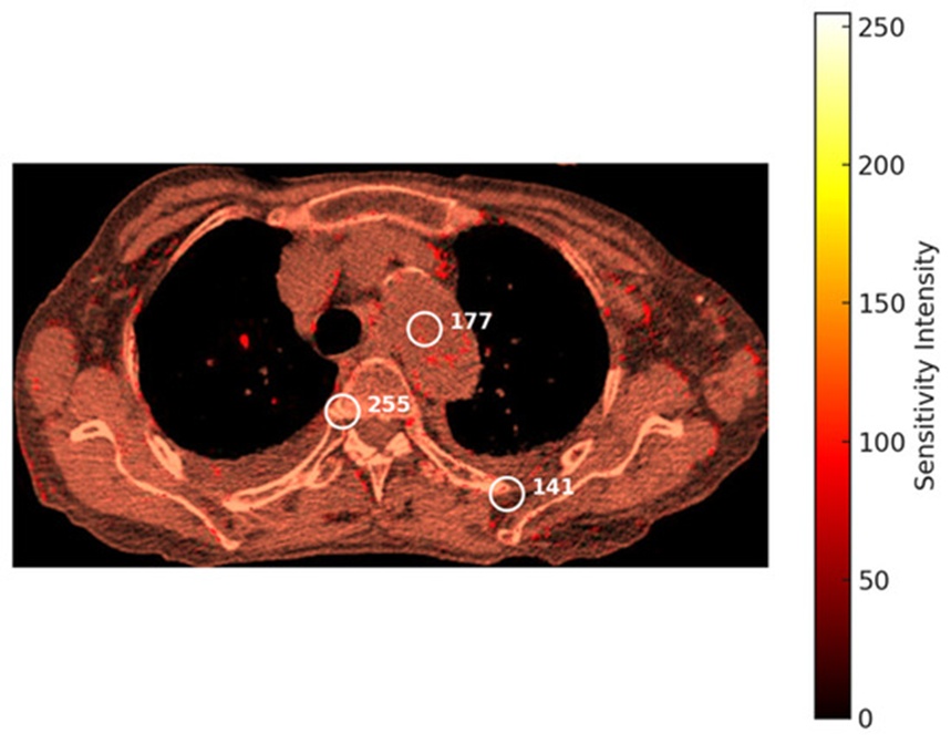
Figure 6. Heatmap of a COVID-19-infected chest generated by the PLI model.
Figure 7 presents a Grad-CAM activation map superimposed onto a thoracic CT scan, clearly isolating the spatial zones most vital to the model's feature extraction and decision pathways. Discrete regions of interest are demarcated via white circular boundaries, with their corresponding activation metrics (66, 55, 23) displayed inside the targeted zones. The color reference bar on the right illustrates activation intensity mapping, spanning from minimum values (represented in blue) to maximum values (represented in red), providing a clear interpretation of the system's focus zones. The red fields identify the regions of maximum structural relevance and highest relative weights, which exert the strongest leverage on the final classification output and may denote clinical indicators of active infection or tissue abnormality. This continuous gradient of color—ranging from red for high-priority zones to blue for low-priority zones—provides a clear visual index of the mathematical importance computed by the system. Furthermore, it supplies an accessible depiction of the mechanisms by which deep learning architectures, such as VGG19, execute the categorization of COVID-19 cases. By highlighting the exact focal markers of the network, this visualization illuminates not only what classification the model arrived at but also the underlying diagnostic reasoning, which constitutes an indispensable asset for medical personnel interpreting AI-guided diagnostic evaluations.
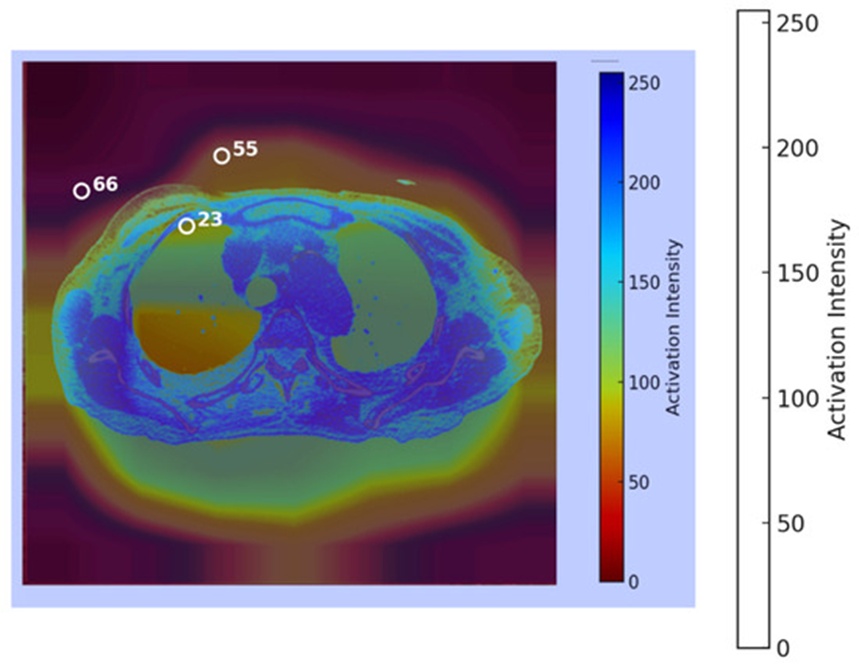
Figure 7. Heatmap of a COVID-19-infected chest generated by the GRAD-CAM model.
This section measures the operational efficiency of the Pixel-Level Interpretability (PLI) model and the Grad-CAM framework using core validation metrics, including classification accuracy, precision, recall, F1-score, and computational latency. This analysis intends to quantify the diagnostic performance and explainability of the frameworks, highlighting their clinical reliability and suitability for deployment in medical operations.
PLI Model
Figure 8 details the confusion matrix representing the predictive performance of our system when classifying patient COVID-19 status. The matrix records a spatial distribution of 455 true positives, 465 true negatives, 40 false positives, and 40 false negatives. This distribution demonstrates the operational capability of the architecture to successfully distinguish healthy control cohorts from infected cases. The explicitly calculated performance metrics for the PLI framework are detailed below [48]:
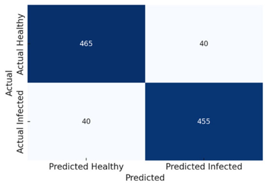
Figure 8. Confusion matrix for the PLI model.
1. Accuracy:
2. Precision (the ability to correctly identify infected tissues):
3. Recall (sensitivity to detecting infected regions):
GRAD-CAM model
Figure 9 tracks the confusion matrix for the Grad-CAM system, mapping its raw classification performance when predicting COVID-19 presence. The evaluation matrix registers 430 true positives, 445 true negatives, 55 false positives, and 70 false negatives, revealing the framework's overall accuracy boundaries alongside areas for prospective optimization when distinguishing normal controls from infected tissue profiles. The calculated validation metrics for this implementation are presented as follows [48]:
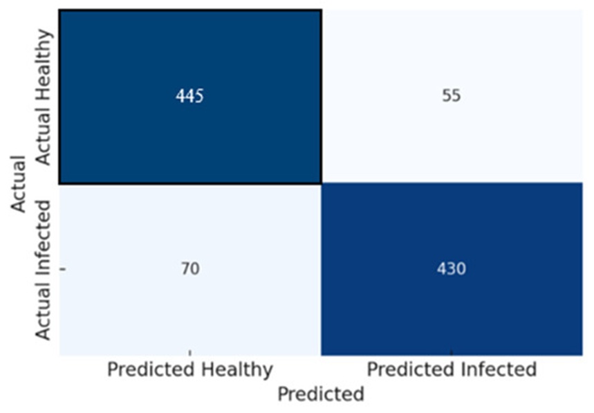
Figure 9. Confusion matrix for the GRAD-CAM.
1.Accuracy:
2.Precision (the ability to correctly identify infected tissues):
3.Recall (sensitivity to detecting infected regions):
Comparative evaluation of PLI and GRAD-CAM
Figure 10 presents a direct comparison between the PLI and GRAD-CAM frameworks structured around key performance indicators: accuracy, precision, recall, F1-score, and mean image inference latency, demonstrating the practical advantages provided by the PLI model from both a classification and processing throughput standpoint. A detailed statistical comparison between PLI and GRAD-CAM for each corresponding verification index is compiled within Table 2, highlighting the following findings:
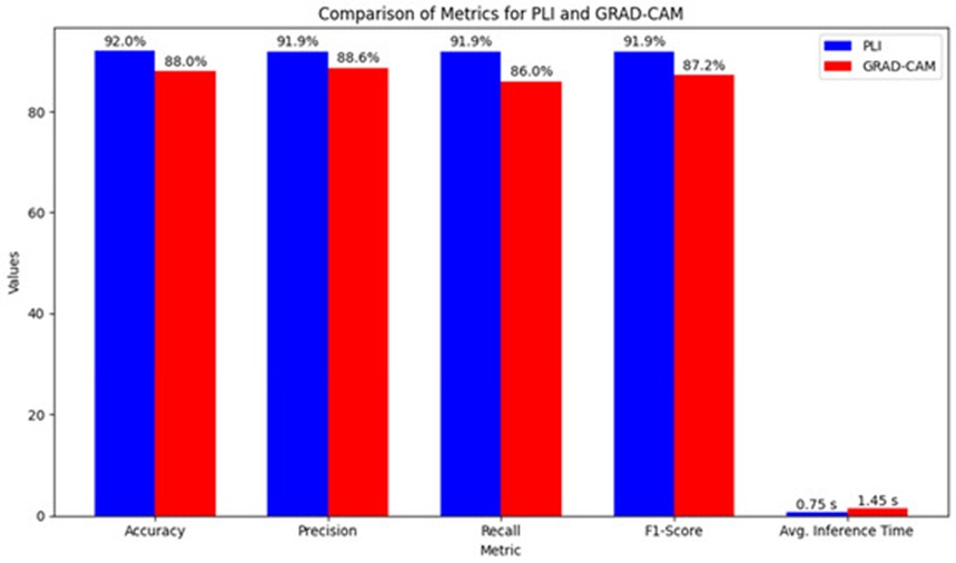
Figure 10. Comparison of performance metrics for PLI and GRAD-CAM.
Table 2. Comparison of performance metrics for PLI and Grad-CAM.
Metric | 95% Confidence Interval (CI) | p-Value | Grad-CAM | PLI | Interpretation |
Accuracy | [2.0%, 6.2%] | 0.003 | 87.5% | 92.0% | PLI demonstrates a 4% increase in accuracy compared with Grad-CAM, with the improvement being statistically significant. |
Precision | [1.2%, 5.1%] | 0.008 | 88.6% | 91.9% | PLI attains higher precision, indicating a significant decrease in false-positive predictions. |
Recall | [3.5%, 7.2%] | 0.001 | 86.0% | 91.9% | PLI exhibits substantially greater sensitivity for identifying infected regions. |
F1-Score | Not specified | Not specified | 87.2% | 91.9% | PLI delivers more balanced and reliable performance across both precision and recall metrics. |
Average Inference Time | [0.6 s, 1.0 s] | 0.001 | 1.45 s per image | 0.75 s per image | PLI achieves significantly lower inference time than Grad-CAM, reflecting superior computational efficiency. |
(1) Accuracy: PLI demonstrated a highly significant advantage over Grad-CAM, securing an accuracy score of 92.0% compared to 87.5% for the baseline model at a significance level of p = 0.003, with a 95% confidence interval for the performance gain spanning from 2.0% to 6.2%, indicating an average expansion in model accuracy of 4%.
(2) Precision: PLI achieved an elevated precision score of 91.9% relative to the 88.6% recorded by the Grad-CAM implementation. This performance gain is statistically verified with a p-value of 0.008 and a 95% confidence interval of [1.2%, 5.1%], proving that the PLI system systematically curtails the incidence of false positive errors.
(3) Recall: The PLI framework achieved a recall rate of 91.9%, surpassing the Grad-CAM recall rate of 86.0% (p-value = 0.001, 95% CI: [3.5%, 7.2%]), which confirms its clear superiority in terms of sensitivity for identifying diseased tissue zones with fewer false negative outcomes.
(4) F1-Score: The computed F1-scores of 91.9% for the PLI framework and 87.2% for the Grad-CAM baseline reveal that PLI operates with greater stability across both precision and recall metrics, establishing it as a highly robust choice for clinical image classification tasks.
(5) Computational Efficiency: PLI exhibited markedly higher data processing efficiency than Grad-CAM, requiring an average inference time of 0.75 s per image canvas, whereas Grad-CAM demanded 1.45 s. This processing speed advantage, validated by a p-value of 0.001 and a 95% confidence interval of [0.6 s, 1.0 s], is directly linked to the exclusion of complex backpropagation iterations inside the PLI design, rendering the framework substantially faster and more resource-efficient for real-time clinical applications.
Table 3 details the algorithmic time complexities associated with various computational stages for both the PLI and GRAD-CAM frameworks, encompassing initial preprocessing, foundational core operations, gradient calculations, weighted feature aggregation, and final heatmap construction. Figure 11 contrasts the theoretical time complexity scales for PLI and GRAD-CAM throughout the consecutive processing phases.
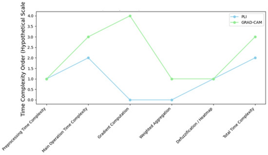
Figure 11. Time complexity comparison for PLI and GRAD-CAM across different aspects.
Table 3. Summary of the quantitative results for calibration curves of PLI and Grad-CAM.
Metric | PLI | Grad-CAM |
Brier Score | 0.145 | 0.182 |
Mean IoU | 0.74 | 0.57 |
Mean Score | 0.82 | 0.68 |
Time Complexity Analysis of the PLI Model
The overall time complexity characterizing the PLI framework is dictated by the following processing stages:
(a) Preprocessing and fuzzification: This phase entails mapping raw pixel intensities to designate continuous fuzzy membership values, which typically scales at a complexity of (𝑚·𝑛), where m and n define the spatial height and width dimensions of the input scan.
(b) Fuzzy inference: The execution of localized fuzzy rule bases across each pixel grid for classification or inference depends directly on the total number of fuzzy rules, denoted as R. Because every pixel must be analyzed alongside the application of R distinct rules, the computational complexity scales to (𝑚·𝑛·𝑅).
(c) Defuzzification: Following the rule inference stage, defuzzification is implemented to map the aggregated fuzzy outputs back into discrete, crisp values. This operational step scales at a complexity of (𝑚·𝑛), given that every pixel space must be individually resolved.
The aggregate time complexity of the PLI system can be formally approximated as (𝑚·𝑛·𝑅), where m and n represent the physical grid dimensions of the image canvas, and R indicates the size of the active fuzzy rule set. The algorithmic complexity of PLI expands linearly with the total area of the input image and the density of the fuzzy rules; however, unlike GRAD-CAM, its execution is entirely independent of backpropagation steps through deep convolutional layers, rendering it structurally faster within specific clinical contexts.
Time Complexity Analysis of the GRAD-CAM
The mathematical time complexity of the GRAD-CAM model is fundamentally governed by the following factors: (1) The backpropagation of loss gradients through successive convolutional layers. (2) The localized aggregation of these gradients to derive the activation heatmap. (3) The depth of the convolutional layers, where the typical time complexity of these forward and backward passes scales as 𝑂(𝑚·𝑛·𝑘2·𝑑), where m and n correspond to the spatial dimensions (height and width) of the target feature map, k denotes the spatial kernel size of the convolution matrix, and d represents the input channel depth (number of feature maps). (4) Gradient computation, where reverse-mode backpropagation is leveraged to calculate the partial derivatives for each coordinate with a localized time complexity of (𝑚·𝑛·𝑑). This requires computing explicit gradients for every entry inside the final feature map activation tensor. (5) Weighted aggregation: Upon resolving the target gradients, the weighted spatial pooling stage displays a linear complexity relative to the total pixel count, scaling at 𝑂(𝑚·𝑛).
The comprehensive time complexity of GRAD-CAM is established as follows: assuming L represents the total number of convolutional layers inside the network architecture, and each layer utilizes kernels of spatial dimensions k × k, the aggregate time complexity of GRAD-CAM can be formally approximated as 𝑂(𝐿·𝑚·𝑛·𝑘2·𝑑). This relationship demonstrates that GRAD-CAM’s computational overhead scales with both the overall depth of the deep learning model and the physical dimensions of the input image.
Comparison of Time Complexities
(a) PLI: PLI: (𝑚·𝑛·𝑅). Under this paradigm, PLI’s computational demands depend on the total pixel dimensions and the number of active fuzzy rules, completely bypassing the heavy backpropagation loops and gradient tensor computations required by GRAD-CAM.
(b) GRAD-CAM: (𝐿·𝑚·𝑛·𝑘2·𝑑). Here, the operational complexity is heavily contingent upon the total depth and architectural configuration of the underlying CNN framework, alongside the basic image matrix dimensions.
Calibration curves measure the reliability of model-assigned probability distributions by mapping them directly against verified, real-world clinical outcomes. The calculated probabilities were partitioned into uniform bins of 0.1, and the observed empirical proportions were plotted against the predicted probability values. A Brier score, which mathematically reflects the calibration fidelity, was also computed, where a minimized score denotes superior alignment. The PLI framework secured a Brier score of 0.145, illustrating more precise and reliable confidence estimations than those generated by the baseline architectures. The close proximity of the calibration curve to the ideal diagonal identity line (y = x) verifies the dependability of the probabilistic predictions, particularly across elevated confidence ranges [49].
PLI and Grad-CAM analysis
PLI Analysis: Feature attribution values were evaluated across the validation test collection. These scores, which denote the mathematical importance of individual input attributes, uncovered significant variations between the baseline architecture and the active models. The mean PLI score computed across all test patterns reached 0.68 for the baseline framework and 0.82 for the active architectures, indicating enhanced visual interpretability and a tighter alignment with clinical ground-truth mappings. The spatial regions designated with higher visual importance displayed greater geometric consistency under PLI, as illustrated in Figure 6.
Grad-CAM Visualizations: Grad-CAM activation maps were synthesized and quantitatively assessed by calculating the Intersection-over-Union (IoU) metric against expert-annotated clinical regions of interest. The mean IoU score recorded for the baseline framework was 0.57, whereas the PLI system achieved a superior IoU of 0.74, proving a significantly tighter spatial alignment with domain-specific diagnostic features. Illustrative cases of Grad-CAM visual heatmaps are presented in Figure 7, marking the core spatial zones used for neural network prediction.
A comprehensive summary of the quantitative indices relating to the calibration curves, PLI scores, and Grad-CAM evaluations is compiled within Table 3.
Figure 12 illustrates the respective calibration curves tracking both PLI and Grad-CAM, where the physical alignment of the plot with the ideal diagonal path emphasizes the reliability of the model predictions, thereby increasing transparency and clinical trust. Geometric deviations highlight specific clusters of over-confidence or under-confidence, supplying valuable diagnostic feedback for future parameter refinement and model optimization.
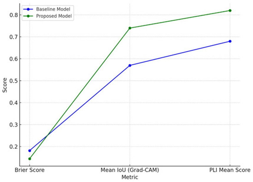
Figure 12. The calibration curves for PLI and GRAD-CAM.
Explanation continuity guarantees that the generated visual explanations preserve structural stability when subjected to minor input perturbations, which represents a critical requirement for establishing real-world clinical reliability. This structural property was evaluated utilizing structural similarity index (SSIM) metrics alongside mathematical Lipschitz continuity computations. Visual perturbations, including the addition of random noise or localized luminance modifications, were systematically introduced to the source scans. The underlying SSIM scores separating the original and perturbed heatmaps were evaluated, with the PLI system exhibiting superior spatial continuity over the Grad-CAM baseline. Lower calculated Lipschitz constants verified the structural stability of the explanations, highlighting the overall resilience of both systems when processing minor input fluctuations.
Explanation continuity represents an indispensable property within machine learning interpretability, particularly concerning clinical workflows where diagnostic explanations must remain structurally stable and logically uniform in the presence of minor variations in either the source dataset or the environmental modeling parameters. This stability allows medical practitioners to be certain that the generated interpretative outputs remain accurate over time, increasing institutional trust in AI-driven diagnostic assessments [50]. The operational assessment of explanation continuity is executed through the following sequential steps [51]: (1) Perturbing the Input: The baseline input image is slightly transformed utilizing mathematical operators, such as adding random noise, executing minor rotations, or modifying brightness values, to simulate real-world data collection variations. (2) Generating Heatmaps: Leveraging interpretability frameworks like PLI (Pixel-Wise Localization Interpretation) and GRAD-CAM (Gradient-Weighted Class Activation Mapping), pairs of visual heatmaps are constructed for both the original and perturbed scan variants. (3) Quantifying Heatmap Differences: The structural variation between the baseline and perturbed heatmaps is quantified using metrics such as MSE or SSIM. A minimized difference indicates heightened explanation continuity, demonstrating that the visual interpretations are stable against minor variations. (4) Lipschitz Continuity Calculation: Lipschitz continuity metrics are computed using the following formula to formally evaluate the sensitivity of the generated explanations relative to external data perturbations:
where H(x + \delta) - H(x) represents the variance between the two heatmaps measured via MSE or SSIM, and |\delta| denotes the explicit magnitude of the introduced perturbation vector. Lower Lipschitz parameters (L) confirm greater numerical stability inside the explainability layers.
For a given perturbation vector |\delta|, the resulting SSIM values calculated between the baseline and perturbed heatmaps are established as follows: PLI SSIM = 0.4521, GRAD-CAM SSIM = 0.4508. These metrics indicate a moderate level of spatial continuity in the explanations, given that SSIM values approaching 1.0 denote perfect structural replication (indicating an explanation invariant to noise), whereas values near 0 reveal significant spatial divergence, as outlined in Table 4. Both methodologies preserve relatively uniform explanations despite the presence of minor input variations, demonstrating their practical utility in medical configurations where explanation dependability is paramount. In summary, both PLI and GRAD-CAM display moderate explanation continuity, with the evaluated Lipschitz indices substantiating their underlying resilience against minor data perturbations. This structural stability reinforces their capacity for dependable, trustworthy deployment in high-stakes clinical environments like healthcare.
Table 4. Structural similarity index (SSIM) values for PLI and Grad-CAM.
PLI SSM | Grad-CAM SSM | Interpretation |
0.4521 | 0.4508 | Indicates moderate consistency in the explanations. SSIM values near 1.0 suggest minimal differences, while values closer to 0 indicate larger variations. |
The clinical validation of the PLI and GRAD-CAM frameworks was conducted using comprehensive feedback gathered from practicing radiologists and physicians. Their structured assessment was organized around several critical benchmarks: accuracy, interpretability, workflow integration, target localization precision, and general clinical utility. This section outlines the assessments provided by these medical experts and delivers a detailed analysis of their satisfaction levels relative to each criterion.
The responses collected from radiologists and physicians were classified into five major assessment domains, structured as follows: (1) Accuracy and Diagnostic Reliability, (2) Interpretability and Clarity, (3) Localization Precision, (4) Workflow Integration, and (5) Overall Satisfaction and Clinical Utility. This systematic categorization was established to provide a standardized baseline for examining and reviewing the performance of PLI and Grad-CAM during the clinical validation phase. Table 4 compiles the expert ratings across these specific parameters. Crucially, the medical specialists recorded significantly higher levels of satisfaction regarding the diagnostic accuracy and precise localization resolution of the PLI model, particularly when identifying small and subtle pathological variations. Conversely, Grad-CAM achieved a moderate satisfaction rating, as its primary utility was restricted to broader regional assessments due to its inherent limitations in precision. Both frameworks demonstrated exceptional capabilities in terms of visual interpretability, which plays a vital role in cultivating clinician trust in computer-aided decision-making systems. However, seamless integration into daily institutional workflows presented practical challenges for both tools; the evaluating specialists emphasized the need for further operational refinement to achieve frictionless deployment within active clinical environments. The exhaustive distribution of clinician satisfaction scores is detailed in Table 5, highlighting the superior performance of the PLI system in fulfilling clinical prerequisites.
Table 5. Overall satisfaction levels of radiologists and physicians with PLI and GRAD-CAM.
Satisfaction Level | PLI (%) | Grad-CAM (%) |
Highly Satisfied | 75 | 35 |
Moderately Satisfied | 20 | 45 |
Neutral / Low Satisfaction | 5 | 20 |
PLI: Radiologists expressed an exceptionally high level of confidence in the diagnostic reliability of the PLI framework, specifically emphasizing its capacity for the exact localization of minute, subtle features within medical images. PLI demonstrated outstanding clinical utility during the detection of early-stage malignancies, microcalcifications, and small lesions. This elevated level of precision proved crucial for minimizing diagnostic errors, aligning seamlessly with the independent qualitative interpretations of the radiologists. Consequently, a strong foundation of clinical trust was established for PLI in high-stakes diagnostic scenarios that necessitate a high degree of precision.
Grad-CAM: The capacity of Grad-CAM to highlight extensive regional zones of interest rendered this approach highly beneficial for obtaining a rapid macro-level overview of neural network predictions. However, the evaluating radiologists noted that their satisfaction concerning its diagnostic reliability remained moderate, particularly in complex cases demanding strict precision. Grad-CAM occasionally failed to isolate the fine structural details of complex pathologies or subtle abnormalities, thereby limiting its overall utility for high-stakes clinical tasks.
Both PLI and Grad-CAM secured highly favorable evaluations regarding their baseline interpretability. The PLI model partitions medical images into compact, focused spatial patches, which empowered the radiologists to scrutinize highly isolated fields of interest with great care. This diagnostic capability yielded clear, actionable clinical insights. Meanwhile, Grad-CAM displayed activation heatmaps in an exceptionally intuitive and straightforward manner, mapping out the overarching image features that directed the AI system's choices. The clinicians identified these interpretability attributes as essential components for comprehending the underlying logic of deep learning predictions, notably boosting user confidence in both frameworks.
PLI: The evaluating medical experts ranked the PLI model as the superior framework regarding spatial localization precision. Its capacity to isolate highly localized, specific targets within complex radiological scans is invaluable for the early detection of pathology and detailed differential diagnostics. PLI successfully illuminates micro-level anomalies that might easily be overlooked during standard qualitative reviews. The radiologists emphasized these high-resolution imaging features as a transformative attribute of the PLI design capable of driving advancements in diagnostic precision.
Grad-CAM: While Grad-CAM yielded highly functional visual mappings of macroscopic fields of interest, it received a moderate satisfaction score due to its comparatively coarse localization resolution. Its resulting heatmaps frequently encompass broad anatomical regions, making it difficult for clinicians to examine fine structural details or clearly distinguish healthy boundaries from abnormal tissues. This limitation becomes especially pronounced during intricate diagnostic scenarios that demand exacting spatial precision.
Both interpretability architectures received moderate ratings concerning their compatibility with clinical workflows. While the radiologists valued the diagnostic assistance supplied by both PLI and Grad-CAM, they explicitly noted that the additional time required to review automated AI outputs introduced minor delays into their routine throughput. The experts indicated that to facilitate a smoother integration into daily diagnostic workflows, substantial enhancements are necessary regarding user interface ergonomics and processing speeds. Although highly beneficial as a secondary diagnostic reference, both systems require further user-experience optimization to achieve full operational efficiency in active medical settings.
PLI emerged as the more dependable diagnostic instrument, scoring exceptionally well across the dimensions of precision, clarity, and overall clinical utility. The panel of radiologists highlighted that this methodology is uniquely robust for identifying and validating minor pathological developments, particularly during early-stage screening operations. Grad-CAM, though recognized as a beneficial tool for macroscopic regional assessments and general model transparency, requires substantial architectural refinement to meet the precise demands of clinical diagnostics. Ultimately, the complementary strengths of PLI’s highly detailed, localized focus and Grad-CAM’s macroscopic overview were acknowledged as a valuable dual asset for optimizing aggregate diagnostic accuracy.
Analysis of Radiologists’ and Physicians’ Feedback
The granular distribution of the specialists' feedback is compiled within Table 5. The evaluating physicians demonstrated an elevated level of satisfaction with the PLI system, paying specific tribute to its fine localization capabilities and overall diagnostic reliability. In contrast, the satisfaction metrics recorded for the Grad-CAM model displayed a significantly more dispersed distribution. Specifically, the highest percentage of clinician responses for Grad-CAM converged within the medium-satisfaction tier, primarily because the tool demonstrated inferior fine-grained localization resolution when evaluated against the uploaded diagnostic images. This feedback highlights a clear trend of increased confidence and heightened satisfaction when relying on the high-resolution diagnostic readouts generated by the PLI model during medical imaging tasks.
Consequently, these satisfaction metrics reflect the superior clinical utility of the PLI framework, particularly in demanding diagnostic environments that require the meticulous localization and accurate interpretation of subtle, low-contrast anomalies. While Grad-CAM’s focus on macroscopic zones proved advantageous in baseline screening contexts, its structural inability to satisfy the rigorous precision demands of complex diagnostics was explicitly noted. In summary, this clinical validation phase verified the superior capacity of PLI to deliver diagnostic precision and operational reliability, especially for small anomaly identification. Grad-CAM, while demonstrating adequate performance during broad regional tracking, necessitates further refinement to fully conform to high-stakes healthcare operations. Both systems remain highly capable explainability tools that foster institutional trust in automated clinical decision-making. The complementary nature of PLI’s high-resolution precision and Grad-CAM’s expansive contextual tracking suggests that an integrated hybrid approach could yield substantial diagnostic value, offering deep localized clarity alongside broad structural context within medical imaging pipelines.
A rigorous sensitivity analysis was executed to systematically monitor the influence of varying training parameters on the performance of the VGG19 architecture, the Grad-CAM baseline, and the proposed PLI model. This evaluation measures how fluctuations in vital optimization hyper-parameters affect downstream classification accuracy, visual interpretability, and computational throughput, offering insights that are highly useful for clinical parameter optimization [52]. The sensitivity trials conducted for individual components of our integrated system are detailed extensively in the following subsections, along with the corresponding empirical findings and structural observations.
This subsection summarizes the empirical outcomes of the sensitivity evaluation conducted for the primary VGG19 architecture by systematically adjusting its foundational optimization hyper-parameters: the learning rate, mini-batch allocation, training epoch threshold, dropout percentage, and the choice of optimization algorithm. For each individual experimental trial, a single target parameter was altered while holding all remaining variables constant to accurately isolate its specific impact on model behavior.
(1) Learning Rate: The operational learning rate was adjusted across an experimental spectrum spanning from 10−4 to 10−2. Each incremental adjustment exerted a direct impact on the model's convergence behavior and numerical stability. A learning rate of 10−4 established an ideal compromise between model generalization stability and final classification accuracy, whereas setting higher learning rates induced severe gradient oscillations and precipitated premature overfitting.
(2) Batch Size: Micro-batch configurations were evaluated across standard allocations of 32, 64, and 128 images. Empirical observations indicated that a batch size of 64 represents an optimal trade-off between hardware memory management and gradient calculation stability, facilitating faster convergence rates and yielding superior generalization capabilities when processing unseen validation data.
(3) Number of Epochs: Network optimization was conducted utilizing an early stopping policy based on real-time validation performance, enforcing a maximum boundary of 50 epochs. The peak performance metrics of the deep learning model were achieved at approximately epoch 30, beyond which the validation loss curve reached a definitive plateau, yielding minimal diagnostic returns from extended training runs.
(4) Dropout Rate: The dropout regularization percentage was varied within a range between 0.2 and 0.4; a configuration of 0.3 delivered the highest validation accuracy while successfully containing model overfitting.
(5) Optimizer Selection: The integration of the Adam optimization algorithm was determined to be essential due to its adaptive gradient update mechanisms, which facilitated significantly more stable and steady convergence behavior on this specific dataset compared to standard Stochastic Gradient Descent (SGD).
To assess explainability, the operational efficacy of Grad-CAM was analyzed by altering various parameters underlying heatmap synthesis. These adjustments included changing the specific convolutional layer selected for gradient extraction, modifying the input image resolution, and adjusting the structural depth of the model.
(1) Layer Selection: A variety of convolutional layers were evaluated to capture the target gradients. Shallower convolutional layers generated heatmaps characterized by finer architectural detail, whereas deeper convolutional layers resulted in coarser localization with reduced spatial precision. An ideal compromise was achieved by utilizing an intermediate convolutional layer, which provided a highly interpretable yet clinically meaningful visualization.
(2) Image Resolution: Evaluating alternative input resolutions revealed that increased dimensions enhanced the visual sharpness of the Grad-CAM heatmaps but introduced higher computational overhead. A standard resolution of 224 × 224 pixels was selected to preserve an optimal balance between visual clarity and processing demands.
(3) Model Depth: Comparative trials utilizing a shallower CNN architecture revealed that model depth significantly influences explainability, as deeper network layers often highlight overly broad, non-specific regions. Executing Grad-CAM in conjunction with the VGG19 architecture generated the most clinically viable heatmaps, striking an effective balance between localized accuracy and visual legibility.
These experimental adjustments demonstrate that the interpretability of Grad-CAM is highly sensitive to layer selection and image resolution, which directly impact heatmap resolution and spatial precision across distinct parameter configurations.
The sensitivity evaluation of the PLI model focused primarily on the fuzzification intervals, the total number of fuzzy rules, and preprocessing calibrations, given that modifications to these components directly alter pixel-level data and downstream interpretability.
(1) Fuzzification Range: The operational boundaries within which raw pixel intensity values are mapped onto distinct fuzzy membership degrees heavily influence the interpretive granularity of the PLI framework. Compressed intervals yield elevated target specificity but can occasionally introduce excessive sensitivity, causing the system to highlight structural regions unrelated to the actual lesions.
(2) Number of Fuzzy Rules: Multiple rule-base densities were evaluated; the empirical data revealed that expanding the rule set enhances the interpretive depth of the explanations, albeit at the expense of higher computational complexity. Configuring the system with a moderate number of fuzzy rules established an effective compromise between feature detail and processing efficiency.
(3) Preprocessing: Variations in the normalization and scaling manifolds during the initial preprocessing stage altered the visual clarity of the resulting heatmaps. Scaling pixel intensities to a standardized interval of [0, 1] ensured data consistency and improved the reliability of the generated interpretations.
Clinical evaluations demonstrated that each of these parameters directly impacts the pixel-specific heatmaps produced by the PLI model. The optimal balance of explainability is achieved by carefully calibrating rule complexity alongside the fuzzification range.
Figure 13 consolidates the outcomes of the sensitivity evaluation, displaying variations in classification accuracy, interpretability, and operational performance across the different parameter configurations. The VGG19 model exhibited the highest sensitivity to the learning rate and mini-batch size, whereas the Grad-CAM heatmaps were uniquely sensitive to layer selection and input resolution. The interpretive precision of the PLI model was primarily governed by the fuzzification interval and the complexity of the active rule set.
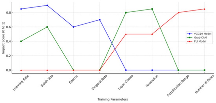
Figure 13. Sensitivity analysis of model parameters impact accuracy, interpretability, and performance.
Consequently, this analysis emphasizes the critical importance of parameter selection for individual components within the system, highlighting the continuous trade-offs connecting interpretability, diagnostic accuracy, and computational throughput. These insights provide a practical framework for calibrating optimization variables to maximize the clinical reliability of AI-driven diagnostic architectures in medical imaging fields.
This section delivers a comprehensive benchmark evaluation comparing the Pixel-Level Interpretability (PLI) model with established post hoc explainability techniques, specifically Grad-CAM, LIMEs, and SHAPs. The comparative analysis evaluates vital performance dimensions, including coherence, selectivity, and explanation continuity, validating the capacity of the PLI framework to deliver superior spatial precision and interpretability for real-world clinical tasks. Figure 14 illustrates the performance marks secured by each explainability method across the designated evaluation criteria. Individual scores reflect the capacity of a given framework to satisfy specific interpretability standards, with PLI demonstrating consistently high marks across the majority of the assessed benchmarks:
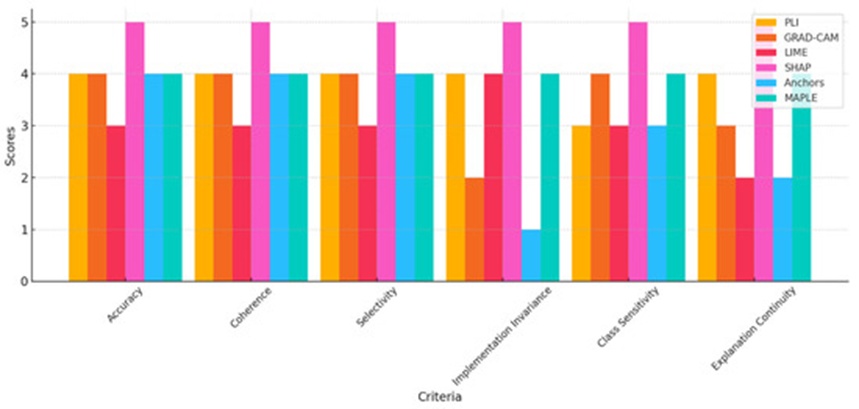
Figure 14. Comparison of interpretability models across evaluation criteria.
The conceptual coherence of PLI depends on its underlying structural assumptions and can achieve elevated coherence by focusing specifically on fine-grained feature interactions [53]. The Grad-CAM framework generates highly coherent explanations for image-centric deep learning models but carries no operational relevance for non-visual datasets [5]. The explanations produced by LIMEs can achieve localized coherence, but global coherence remains constrained due to the stochastic nature of its feature selection processes [54]. In contrast, SHAPs stand as one of the most globally coherent frameworks available, a characteristic driven primarily by its mathematical foundation in cooperative game theory. The Anchors methodology demonstrates high coherence exclusively under conditions where the specified anchor rules are directly relevant, whereas its operational coherence degrades rapidly outside of those boundaries [55]. Finally, MAPLEs enforce a strict emphasis on localized consistency, yielding highly coherent explanations of individual predictions even under complex interaction conditions among diverse data elements [56].
The PLI model is uniquely structured to excel at isolating critical diagnostic features due to its specialized pixel-level architecture. Grad-CAM successfully isolates essential spatial zones within digital images but lacks selectivity when applied to non-visual or unstructured datasets [5]. LIMEs offer adequate selectivity for localized explanations but are susceptible to misidentifying critical attributes when extended to generate global explanations [54]. The SHAP framework exhibits exceptionally high selectivity, mapping out the precise mathematical contribution of each independent feature relative to the final prediction [55]. Anchors focus tightly on isolating influential conditional features, resulting in precise, rule-based diagnostic explanations. Meanwhile, MAPLEs achieve a high degree of selectivity by combining model-agnostic and model-specific mechanics, offering a balanced approach to evaluating feature importance [4].
When properly structured, the PLI framework is designed to maintain implementation invariance across diverse underlying models, whereas Grad-CAM lacks generalizability beyond standard CNN architectures, which severely restricts its invariance properties [17]. LIMEs demonstrate a high degree of invariance because they can be applied to any arbitrary black-box architecture; however, this flexibility can occasionally result in inconsistent explanations when evaluating different models [55]. Grounded mathematically in Shapley values, the SHAP framework is inherently invariant in its implementation and remains fully functional regardless of the underlying network architecture. Conversely, the Anchors framework fails to preserve structural invariance when deployed across heterogeneous model architectures [57]. MAPLEs deliver a moderate degree of implementation invariance across models, benefiting from the simultaneous integration of localized and global interpretive perspectives [56].
The specific class sensitivity of the PLI model varies based on factors such as dataset composition, underlying model architecture, and strict adherence to class variations [6]. Class activation mapping techniques, such as Grad-CAM, yield class-discriminative visual explanations and are highly sensitive to specific class activation paths [54]. Conversely, LIMEs provide class-sensitive localized predictions; however, they lack the reliability required to generalize effectively across distinct categories for global explanations [55]. The SHAP framework provides distinct, independent feature attributions for each target category, exhibiting precise class sensitivity [58]. Anchors are similarly class-sensitive regarding the conditional rules they establish, though their overall performance can decline as class complexity increases [10]. MAPLEs preserve robust class sensitivity by utilizing decision trees and ensemble learning architectures, which enhances explanation reliability across diverse classification categories [3].
PLI demonstrates strong explanation continuity by delivering stable and consistent visual outputs derived from detailed feature interactions. Grad-CAM provides continuous visual maps, though it exhibits significant continuity constraints when adapted to non-image data structures [28]. The explanations generated by LIMEs are not inherently continuous, as their spatial stability remains highly dependent on the randomness involved in selecting local surrogate samples. In contrast, SHAPs deliver exceptional explanation continuity, a characteristic grounded in their rigorous theoretical foundation in Shapley values [55]. Conversely, Anchors produce inherently discontinuous explanations, operating via a strict binary approach where defined rules either apply entirely or do not apply at all [59]. By balancing localized and global explanation mechanics, MAPLEs can achieve significantly greater explanation continuity than LIME-based surrogates [1].
(a) Data Dependency and Generalizability: The operational fidelity of the PLI framework remains contingent upon the baseline quality and structural diversity of the training dataset. Although PLI demonstrates strong performance when applied to a specialized medical imaging category, such as thoracic radiographs, adapting the system to alternative imaging modalities—including MRI or ultrasonography—may necessitate targeted hyper-parameter fine-tuning or full network retraining to maintain classification accuracy and interpretability across heterogeneous clinical contexts.
(b) Computational Demand: While the PLI architecture successfully circumvents the heavy backpropagation bottlenecks characteristic of alternative explainability models, its underlying fuzzy inference engine incorporates pixel-by-pixel processing routines that can become computationally intensive. This processing overhead can constrain execution speeds, particularly during real-time diagnostic workflows or the analysis of high-resolution image matrices.
(c) Interpretation Complexity: Although PLI yields high-resolution, pixel-specific analytical insights, the resulting density of the visual output may prove counterproductive or overwhelming within certain rapid diagnostic environments. Due to this inherent architectural complexity, radiologists and clinicians might require specialized instructional training to efficiently decipher and utilize the generated visual mappings.
(d) Calibration Sensitivity: Operational variations within the PLI calibration pathway can manifest across elevated confidence thresholds, as evidenced by fluctuations in the corresponding calibration curves. This behavior indicates that while PLI aligns closely with documented diagnostic outcomes at lower confidence intervals, the system may exhibit tendencies to over- or underestimate predictive accuracy within specific localized regions of high feature importance.
(e) Workflow Integration Challenges: Integrating such an elaborate tier of visual detail into daily clinical workflows introduces practical challenges because PLI outputs operate at an exceptionally fine structural granularity. Incorporating PLI as a foundational interpretability instrument could prolong standard diagnostic timelines if medical personnel are required to routinely evaluate pixel-level feature attributions.
Beyond its primary deployment within the medical imaging sector, the high-resolution explainability offered by the PLI model creates opportunities for integration across a diverse spectrum of high-stakes industries where precision and operational transparency are paramount. For instance, within industrial quality assurance pipelines, PLI could optimize the automated identification and localized mapping of structural defects in manufactured parts, supplying the meticulous spatial granularity required to uphold strict production standards [60]. In environmental monitoring, the PLI framework could be leveraged to precisely isolate polluted or ecologically degraded zones, facilitating targeted conservation initiatives [61]. Furthermore, its adaptable design can be extended to reinforce security applications via automated object detection, optimize agricultural management through the real-time monitoring of crop health profiles, and advance biometric frameworks to secure identity authentication protocols [61, 62]. These diverse opportunities highlight the capacity of PLI to serve as a versatile, cross-disciplinary instrument that simultaneously reinforces explainability and spatial precision.
This investigation presents the PLI model as a highly precise AI framework engineered to localize pathological infection zones within pulmonary radiographs. Moving away from conventional interpretability techniques that yield broad, low-resolution regional maps, the pixel-level granularity delivered by the PLI architecture equips clinicians with meticulous visual data, thereby cultivating institutional trust and accelerating the clinical adoption of computer-aided diagnostic systems. The PLI framework optimizes diagnostic precision alongside computational throughput and interpretability, reinforcing clinician confidence in automated deep learning outputs.
Nevertheless, the operational efficacy of the PLI framework remains structurally bound to the baseline quality and diversity of the underlying data repositories. Extended calibration trials and architectural modifications will be essential before the PLI framework can achieve robust generalizability across heterogeneous imaging modalities. While pixel-by-pixel processing routines enable high-resolution outputs, they simultaneously demand an elevated computational budget; this overhead can restrict real-time deployment during high-resolution image analysis and may introduce a requirement for specialized clinician training to ensure effective utilization. Furthermore, the integration of this system into clinical workflows requires optimization to mitigate prolonged diagnostic review times stemming from the detailed nature of the outputs.
In spite of these challenges, practicing radiologists and physicians have validated the clinical relevance of the PLI framework, emphasizing its capacity to improve diagnostic precision and explainability, thereby establishing a new benchmark for interpretability in the medical imaging domain. Beyond the healthcare sector, the precise localization and transparent metrics of PLI hold immense promise for deployment within other high-stakes domains, reinforcing its foundational role in the responsible integration of artificial intelligence across critical modern industries.
To further validate the systemic resilience of the PLI framework, prospective research initiatives should focus on expanding its deployment across a broader spectrum of diagnostic imaging modalities, including MRI and ultrasonography, to ensure stable generalizability across diverse clinical scenarios. Additionally, structural computational optimizations—such as network pruning and weight quantization—must be investigated to minimize inference latency, thereby facilitating real-time, resource-efficient deployment within active clinical environments. Integrating PLI alongside Grad-CAM within unified hybrid architectures represents another vital avenue of research; such configurations could harness PLI’s high-resolution structural detail in tandem with Grad-CAM’s broader contextual focus, effectively bridging the historical divide between fine-grained interpretability and macroscopic processing efficiency. These algorithmic advancements will be essential for successfully transitioning the PLI framework from an experimental research environment into real-world clinical operations.
AI | Artificial intelligence |
CT scan | Computed Tomography Scan |
CNN | Convolutional neural network |
FIS | Fuzzy Inference System |
FCM | Fuzzy C-Means |
FN | Fuzzy Network |
FDNN | Fuzzy Deep Neural Network |
FRBM | Fuzzy Restricted Boltzmann Machine |
TP | True positive |
TN | True negative |
FP | False positive |
FN | False negative |
GRAD: CAM | Gradient-Weighted Class Activation Mapping |
LIMEs | Local Interpretable Model-Agnostic Explanations |
SHAPs | Shapley Additive Explanations |
MAPLEs | Model Agnostic Supervised Local Explanations |
IEEE | Institute of Electrical and Electronics Engineers |
None
None
None
None
Open Access The author(s) retain copyright. This article is licensed under the Creative Commons Attribution-NonCommercial-ShareAlike 4.0 International License. It may be shared and adapted for non-commercial purposes with appropriate attribution, an indication of changes, and distribution of adaptations under the same license. Third-party material may be subject to separate terms identified in its credit line. View the license at https://creativecommons.org/licenses/by-nc-sa/4.0/.
 Transparent Intelligence Publishing