The climate system is heavily influenced by aerosols through direct and indirect pathways, notably the absorption and scattering of radiant energy. Beyond climate impacts, these particles compromise atmospheric visibility and jeopardize public health. Specifically, human populations face exposure to fine particulate matter PM2.5, a major driver of respiratory and cardiovascular pathologies. Long-term modifications in PM levels are generally governed by emission shifts and meteorological patterns, whereas short-term fluctuations are predominantly dictated by immediate weather dynamics. Surface variations in PM2.5 levels are further driven by environmental variables such as temperature, wind velocity, relative humidity, and vegetative coverage.
Air quality forecasting has advanced significantly through the application of machine learning. This research explores PM2.5 estimation by utilizing these environmental and meteorological metrics as spatiotemporal inputs. This study evaluates seven years (2014–2021) of in situ PM2.5 measurements gathered from five distinct monitoring stations across Singapore, establishing a baseline dataset for spatial modeling.
The primary contribution of this paper is a novel predictive architecture tailored for temporal analysis, utilizing Random Forest (RF), Gradient Boosting (GB) regression, and the Tree-based Pipeline Optimization Tool (TP) Auto ML framework, which optimizes via a meta-heuristic genetic algorithm. The TP model demonstrated strong predictive capabilities, achieving a peak Global Performance Index (GPI) of 7.4 in August 2016 and a minimum value of −0.6 in June 2019. These metrics highlight the robust nature of the TP framework; its negative values remained superior to competing models, indicating less pessimistic errors. Finally, the underlying logic of these machine learning systems is clarified using eXplainable Artificial Intelligence (XAI) methods, which validate the integrity of feature importance and offer deeper insights into the cyclical variations of PM2.5 concentrations.
The inhalation of particulate matter (PM) poses a severe risk to human health, inducing both acute and chronic ailments by compromising the respiratory system. Particulates with an aerodynamic diameter of ≤2.5 µm, classified as PM2.5 , are highly hazardous and are directly linked to respiratory tract damage, lung cancer, and tuberculosis [1, 2]. Even short-term spikes in ambient PM2.5 levels have a destructive impact on public well-being, driving up mortality rates [3-6].
Atmospheric degradation, particularly across Asian territories, is heavily exacerbated by toxic heavy metals embedded within PM2.5 [7]. To quantify these effects globally, Lelieveld et al. [8] simulated PM2.5 distributions via a global atmospheric transport model, pairing their findings with the exposure–response functions established by Burnett et al. [9]. This analytical framework provides the necessary context for estimating worldwide premature mortality stemming from ischemic heart disease (IHD), cerebrovascular disease (CEVD), lung cancer (LC), and chronic obstructive pulmonary disease (COPD) [10].
Over the past few decades, PM2.5 trends have shown highly dynamic patterns of escalation and decline across the globe, with distinct shifts visible in highly industrialized and economically advanced regions [11]. In modeling these trends, Chen et al. [12] integrated various environmental and meteorological predictors—including temperature, wind speed and direction, relative humidity, and vegetative coverage—due to their direct influence on localized surface PM2.5 gradients. Auxiliary spatial metrics, such as the Normalized Difference Vegetation Index (NDVI) used to map forests, water bodies, agricultural fields, urban settlements, and barren terrain, correlate closely with localized emission origins and the atmospheric transport of airborne particles.
A frequent limitation in broad-scale air quality modeling is the scarcity of spatial data from ground-based monitoring networks. To overcome this, researchers leverage satellite observations, which offer the spectral and spatial coverage required for effective PM2.5 forecasting [13]. Aerosol optical depth (AOD) serves as a primary metric for quantifying how effectively aerosols attenuate light within the atmosphere. Because AOD is dictated by the composition, size, and spatial distribution of these particles, combining satellite-derived AOD with meteorological inputs is a standard approach for mapping PM2.5 [14, 15]. Beyond AOD measurements, high-quality reanalysis products are frequently utilized to supply meteorological inputs for PM2.5 models. Prominent examples include the Modern-Era Retrospective Analysis for Research and Applications, Version 2 (MERRA-2) and the European Centre for Medium-Range Weather Forecasts (ECMWF) ERA5 dataset, the latter featuring a spatial resolution of 0.25° × 0.25° [16].
Global land cover inventories (300 m resolution) and MODIS NDVI data (250 m resolution) are also integrated as supplementary inputs for PM2.5 models. The Moderate Resolution Imaging Spectroradiometer (MODIS), operating on the Terra and Aqua satellite platforms, offers several specialized instruments. These include the MODIS Dark Target (DT) and Deep Blue (DB) products, both operating at a 10 km spatial resolution, alongside the MODIS DB Multi-angle Implementation of Atmospheric Correction (MAIAC), which provides a finer 1 km resolution [15, 17]. The utility of MODIS-derived parameters, such as AOD and land surface temperature (LST), in refining the precision of PM2.5 models has been verified by Sekertekin et al. [18] and Xiang et al. [19]. Conversely, traditional spatial interpolation techniques like inverse distance weighting (IDW), when used to fill gaps between ground stations, exhibited a 24% error margin between estimated and observed PM2.5 concentrations across monitoring sites in Delhi [20].
A variety of statistical architectures, such as autoregressive integrated moving averages (ARIMA) and multiple linear regression, have been implemented by Ma et al. [14] to estimate PM2.5 dynamics. To handle data gaps in spatial records, Pu and Yoo [15] engineered a multi-stage modeling framework that quantifies spatial uncertainties to deliver reliable PM2.5 estimations. Because the accuracy of these models is intimately tied to data density, mathematical approaches like the wavelet transform have been deployed to augment dataset completeness [21]. Machine learning (ML) paradigms are uniquely suited for these tasks, as they use specialized training routines to unravel complex, non-linear patterns within data. In environmental science and extreme weather forecasting, ML systems trained on curated benchmark data excel at identifying key feature interactions under diverse atmospheric states [22]. Both statistical formulations and ML frameworks are regularly deployed to assess PM2.5 loads and isolate the localized severity of emissions in vulnerable areas [23].
To optimize the accuracy of time-series meteorological forecasting and map the core characteristics of PM2.5, researchers utilize an array of ML methods. These include Bayesian statistics, standard regression variants, Random Forest (RF), radial basis function long short-term memory (RBF-LSTM) networks, maximum likelihood estimation (MLE), support vector machines (SVM), K-nearest neighbor (KNN) classification, and artificial neural networks (NN) [13, 21, 24]. Furthermore, deep learning (DL) models offer exceptional predictive capabilities when their hyperparameters are properly optimized. Current research also explores how these advanced DL frameworks can be adapted to evaluate particle dispersion problems across broader atmospheric chemistry datasets.
To address the "black box" nature of these models, eXplainable Artificial Intelligence (XAI) has emerged as a vital methodology for evaluating algorithmic transparency and verifying feature reliability [25]. While XAI is increasingly favored for interpreting feature weights and model trustworthiness, certain techniques fail to satisfy ideal theoretical criteria and run into operational constraints. Implementing model-agnostic methods can significantly mitigate algorithmic bias. Nonetheless, many XAI strategies violate core mathematical properties (such as "implementation invariance" or "completeness") and exhibit notable limitations depending on the problem setup. For example, the softmax layer in neural networks generates class weights with probabilistic characteristics, but these do not constitute true mathematical probabilities. In contrast, random forests and random survival forests determine class likelihoods via relative frequencies, calculating exact probabilities based on the actual percentage of distinct sample classes present at each leaf node [26]. Consequently, the fidelity of these class probability distributions is bounded by the volume of training data and the specific ML architecture deployed. Overcoming these limitations remains a major hurdle when designing post hoc interpretability models for opaque systems [27].
XAI techniques are also being actively applied to remote sensing workflows. For instance, Kakogeorgiou et al. [28] applied saliency maps to qualitatively inspect the BigEarthNet and SEN12MS benchmark datasets, which are commonly used to train deep learning models for data imputation. Their evaluation spanned several methods, including Input × Gradient (InputXGrad), Integrated Gradients (IntGrad), Guided Backpropagation (GuidedBackprop), Grad-CAM, Guided Grad-CAM, Occlusion, DeepLift, Lime, and SmoothGrad (SG), ultimately minimizing maximum sensitivity to ensure stable data classification. Similarly, the Shapley Additive Explanations (SHAP) model was used in Israel to interpret diverse spectroradiometric and ecological data (such as the Ecological Spectral Information System and ASD Field Spec bare fiber data) across multiple vegetative scenarios, extracting critical insights regarding leaf area index, nitrogen distribution, and water content [29].
Stadtler et al. [30] leveraged a multi-labeled global air quality benchmark dataset to examine black-box architectures, applying SHAP, Neural Network Activation, Random Forest Activation, and KNN-based error analysis to interpret average tropospheric ozone distributions across distinct intervals. The SHAP framework was likewise chosen by Betancourt et al. [31] and Stirnberg et al. [32] to clarify data contributions and improve algorithmic transparency. These machine learning setups utilized the global AQ-Bench repository and reanalyzed observations (ReObs) from Paris Charles de Gaulle Airport to forecast variations in tropospheric ozone and \text{PM}_1 concentrations. Lastly, the Regression Activation Mapping (RAM) technique was implemented within the Indian wheat belt to assess the step-by-step contribution of individual variables when forecasting satellite-derived vegetative indices and meteorological parameters at a daily temporal resolution.
This investigation undertakes the spatial forecasting of monthly PM2.5 concentrations using satellite observations, supplemented by sparse validation data gathered from monitoring stations distributed across the northern, southern, central, eastern, and western sectors of Singapore. Spatial mapping is achieved through data-driven approaches incorporating aerosol optical depth (AOD) alongside environmental and meteorological predictors. The primary objective of this research is to evaluate multiple ML paradigms for spatial prediction. The secondary objective centers on enhancing spatial PM2.5 forecasting performance by integrating multiple input dimensions and optimizing predictive outputs through ensemble methods and meta-heuristic approaches. Furthermore, this study clarifies the underlying drivers of these predictions by applying advanced XAI methodologies to the various models. The selected ML frameworks—comprising Random Forest regression, the Gradient Boosting regression algorithm, and TP—are trained on AOD data paired with meteorological inputs, including wind dynamics, relative humidity, temperature, and vegetation coverage, to model surface PM2.5. These ML techniques operate on a one-time-step training and prediction framework, successfully generating sequential outputs with high accuracy for subsequent intervals. The architecture is engineered to predict values for every pixel and data point within the study domain, with each output examined via XAI. While recent years have seen extensive exploration of PM2.5 levels using ML, pixel-level spatial forecasting remains an under-researched area. Although several prominent neural network designs have been applied to PM2.5 modeling, they frequently fail to capture peak variations during extreme events [33], and interpreting their internal transparency, uncertainty, and explainability is notoriously difficult. Furthermore, neural networks exhibit a higher propensity to overfit exploratory variables when external factors are introduced [33]. Conversely, ML methodologies are capable of learning high-dimensional, complex representative characteristics [34] while remaining straightforward to interpret. A distinct research gap persists regarding model complexity, interpretability, spatiotemporal dynamics, feature selection and engineering, and the implementation of hybrid or multi-model systems to achieve superior spatial prediction accuracy.
The insights gained from this study, which focuses on various atmospheric pollutants, can assist in formulating mitigation strategies. This objective aligns with efforts to develop inclusive, sustainable, resilient, and safe cities and human settlements. Integrating remote sensing technologies, open-source data products, and statistical methods with XAI-enhanced ML frameworks can substantially increase PM2.5 predictive accuracy and guide optimal air quality management policies. The novelty of this study lies in revealing the capabilities of dynamic ML models that leverage historical records and key parameters to forecast PM2.5 using spatiotemporal satellite datasets and diverse meteorological variables. It also identifies the specific input parameters that strongly dictate PM2.5 forecasts over Singapore based on temporal statistical premises, justifying the requirement for multi-feature inputs and evaluating the internal variations of different tree-based machine learning models with and without optimization routines. The development and deployment of this novel ML framework for mapping spatial PM2.5 distributions and assessing the temporal dynamics of fine particulate matter are guided by the following objectives:
(i) Mapping spatial PM2.5 distributions across Singapore and validating the results through machine learning models.
(ii) Assessing the fidelity of the resulting model predictions via XAI.
Situated at the southernmost tip of the Malay Peninsula, approximately 137 km north of the Equator, Singapore is a highly urbanized city-state populated by 5.7 million residents and 3 million daily commuters [35-37]. Defined by an equatorial climate with persistent year-round precipitation, elevated humidity, and high temperatures, the study focuses on in situ monitoring stations chosen to capture the spatiotemporal dynamics of Singapore's air quality, as illustrated in Figure 1. The National Environment Agency (NEA) of Singapore systematically records ambient air pollutants, including particulate matter (PM2.5 and PM10). As previously noted, PM2.5 denotes finer particulates with an aerodynamic diameter ≤2.5 µm, which are predominantly linked to adverse health outcomes and long-range atmospheric transport [38, 39]. Conversely, PM10 encompasses larger particles with diameters \le 10\ \mu\text{m} [40]. Because of their larger dimensions, their direct health risks are less severe, yet they remain critical components in meteorological and climate processes [41], forest fire monitoring [42], industrial transport tracking [43], and pollution source apportionment [44].
For this investigation, the scope is restricted to PM2.5 metrics [6] recorded at the northern, southern, eastern, western, and central monitoring stations across Singapore (as delineated in Figure 1). The collected data were compiled into monthly averages spanning 2014–2019, focusing specifically on June, July, August, and September, which demonstrate prolonged rainfall deficits relative to the rest of the year.
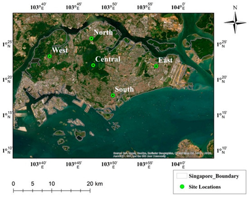
Figure 1. Satellite imagery of study area, Singapore.
The geographic positioning and cartographic representation of the study domain are illustrated in Figure 1, highlighting the five monitoring stations strategically deployed across the western, northern, eastern, southern, and central zones of Singapore to gather empirical observational data.
The operational sequence illustrated in Figure 2 outlines the methodology executed in this research. Spatial datasets from both MODIS and ERA5 were utilized. The Climate Data Store (https://cds.climate.copernicus.eu/, accessed on 24 March 2022) delivers global ERA5 products mapped onto a 0.25° × 0.25° latitude–longitude grid across multiple timescales, representing the fifth generation of the ECMWF atmospheric reanalysis for global climate modeling. For this study, the MODIS platform—encompassing the Terra and Aqua satellites with Collection 6.1, level 2 aerosol optical depth products at a 550 nm wavelength over both land and ocean surfaces [45]—is utilized at a spatial resolution of 10 km.
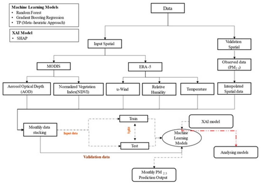
Figure 2. Systematic methodology detailing the data, models, and procedures used.
Python served as the primary programming environment for dataset preparation and ML model execution, while spatial configurations were mapped using ArcGIS 10.3. Preprocessing routines were executed to convert the raw data into an optimized input architecture for model training. The preprocessing sequence in this study involved feature variable selection, missing value imputation to bridge spatial gaps using observational data points, and partitioning the datasets into 70% training and 30% testing subsets for algorithmic assimilation.
Inverse distance weighting (IDW) interpolation was applied to the ground-based observations to validate the spatially predicted model outputs; a representative example is shown in Figure 3. During preprocessing, the input metrics were resampled to a coarse resolution of approximately ~0.25° × 0.25° prior to training the machine learning models. The comprehensive methodology and the specific parameters configured for each technique are presented systematically in Figure 2.
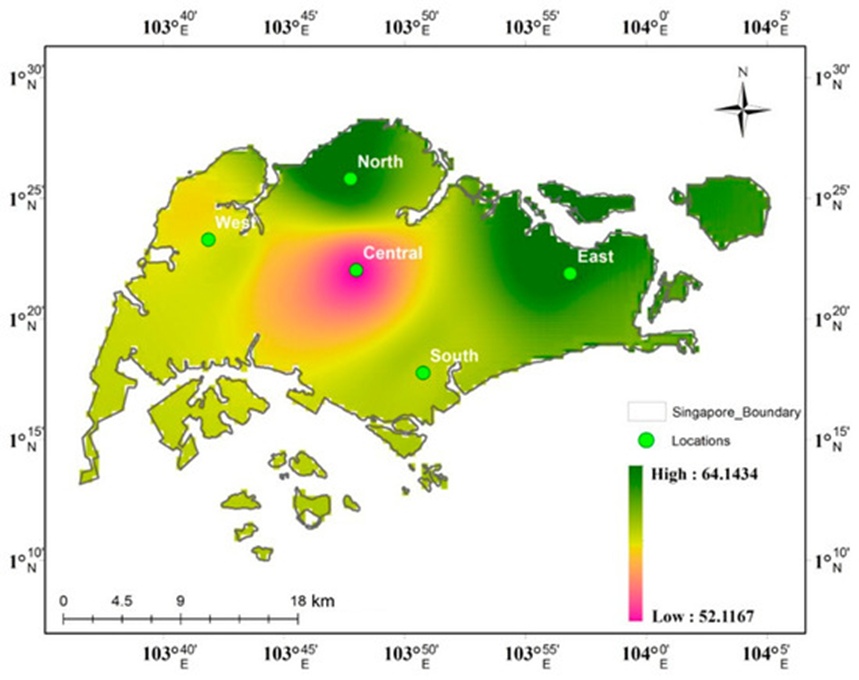
Figure 3. Inverse distance weighted interpolated data using observation data for January 2014 of PM2.5 concentration.
RF is a machine learning paradigm used for both classification and continuous regression tasks. It functions as a bootstrapped, tree-based ensemble method utilizing a bagging mechanism that aggregates numerous decision trees to output highly stable predictions. The random forest framework generates an ensemble of decision trees, where each individual tree is formulated from a distinct subset of training data alongside a randomized subset of features at every node split. Sample generation matches the designated tree count, and tree growth is dictated by the optimal split and node configuration of the input parameters within the dataset [46]. This architectural randomness suppresses overfitting and enhances the generalization capability of the model. The performance of the RF algorithm is primarily governed by two hyperparameters: the total number of decision trees and the feature subset size allocated to each node split.
While expanding the number of decision trees improves model accuracy, it simultaneously scales up the computational demands. The number of features considered at each node split is typically determined by taking the square root of the total feature count within the dataset. This feature count parameter can be adjusted to strike an optimal balance between model bias and variance. For continuous regression problems, the random forest model computes the mathematical mean of all individual regression tree predictions. Each constituent regression tree outputs a constant value for the target variable, and the final prediction generated by the overall random forest is the average of these individual tree forecasts. This aggregation technique reduces overall model variance and elevates predictive accuracy.
Like RF, GB is an ensemble learning paradigm; however, it constructs its decision tree components sequentially rather than in parallel. This supervised methodology integrates two algorithmic elements—decision trees and additive expansion—to synthesize the final predictive output. The GB framework incorporates a loss function to drive output convergence, minimizing predictive errors by iteratively fitting less complex decision trees [47]. Gradient boosting sequentially appends weak learners to the ensemble, with each new learner designed to minimize the residual errors of its predecessors. The trees are explicitly constructed to counteract the deficiencies of the prior model state. At each step, the algorithm computes the negative gradient of a defined loss function relative to the predictions of the existing ensemble, subsequently fitting a new tree to these negative gradients. A major benefit of gradient boosting is its capacity to accommodate diverse loss functions, such as mean squared error for regression tasks and cross-entropy loss for classification applications. It is also highly robust against missing values and data outliers. The operational performance of gradient boosting relies heavily on several hyperparameters, including the learning rate, the number of sequential trees, the maximum tree depth, and regularization factors. The learning rate dictates the marginal contribution of each successive tree to the final prediction; a lower learning rate typically yields superior performance but requires more iterations to converge. The total tree count defines the structural complexity of the ensemble, where a larger number of trees can boost accuracy at the expense of higher computational costs. Tree depth governs the internal complexity of each weak learner, with excessive depth frequently causing overfitting. Finally, regularization parameters, such as the minimum sample threshold per leaf and the maximum allowable depth, serve as vital guardrails to prevent overfitting.
This highly efficient machine learning algorithm implements a Gradient Boosting framework centered on optimized decision-tree structures. This model regularly outperforms alternative architectures when applied to small- to medium-sized datasets. While it requires the configuration of specific hyperparameters, these parameters can be automated to truncate the training process once optimal validation metrics are achieved [48, 49].
Optimization frameworks are generally classified into exact algorithms and heuristic approaches. Heuristic methods are tailored to specific problems, whereas meta-heuristic frameworks encompass broader strategies like the Genetic Algorithm (GA) [50]. Random Search [51], Grid Search, and the Evolutionary Algorithm (EA) [52] represent standard methodologies for engineering AutoML architectures across diverse fields. TP is an AutoML framework engineered to systematically discover optimal machine learning pipelines using a GA, which is a highly effective approach for navigating complex and irregular search spaces [53-55]. In this study, TP evaluates a multitude of randomly generated candidate pipelines [56]. The pipeline design balances model accuracy against structural complexity. TP automates feature selection, feature engineering, model selection, and hyperparameter optimization. Comprehensive cross-validation is performed across the entire pipeline structure based on its cross-validated performance score [57], such as mean squared error or balanced accuracy.
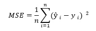
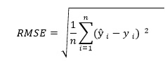
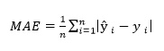
To evaluate the mathematical performance of the regression frameworks and guide model optimization, several diagnostic metrics are calculated. Different validation indicators are suited to specific machine learning tasks; because this study addresses a continuous target estimation problem, model validation is conducted using Mean Squared Error (MSE), Root Mean Squared Error (RMSE), Mean Absolute Error (MAE), Mean Absolute Percentage Error (MAPE), and the PM2.5 coefficient of determination [58-60].
 (1)
 (2)
 (3)
 (4)
 (5)
 (6)
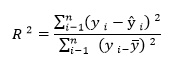
As a standard validation metric, MSE determines the average squared residual between estimated and observed coordinates. To quantify the physical deviation of the model outputs relative to empirical targets, RMSE is computed. Meanwhile, relative absolute variations are normalized via MAPE to provide a percentage-based benchmark for cross-model validation [61]. MSE serves as a core diagnostic tool for auditing ML architectures, measuring the mean of the squared boundaries separating predicted points from true observations. Squaring these residuals ensures that larger predictive errors are assigned a disproportionately higher penalty. RMSE offers an alternative metric that maintains sensitivity to the original data scale, whereas MSE does not account for the baseline scale of the response variables. Consequently, RMSE responds more dynamically than MSE to fluctuations across the target values. The R2 index is widely chosen to define the explained variance within regression structures, representing the percentage of target variable fluctuations successfully captured by the model’s predictor array. Higher R2 scores signify a closer mathematical alignment between the model and the empirical dataset.
The R2 metric is a post-estimation coefficient derived from the residual sum of squares. When the residual sum of squares minimizes toward zero, pushing the final R2 toward 1, it demonstrates that the model completely characterizes the target variable's internal variance; conversely, an elevated error sum of squares indicates a poor regression fit.
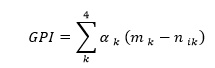
Zhu et al. [62] introduced the Global Performance Index (GPI) as an objective framework for ranking competing machine learning configurations. The GPI aggregates multiple statistical indicators into a singular score to reveal the optimal model setup. The algebraic definition of the GPI incorporates a fixed multiplier αk, set to 1 for metrics where lower values are optimal (such as MSE, RMSE, and MAPE) and assigned -1 for R2. The normalized value of each statistical parameter is expressed as nik, with mk representing the median value of the normalized indicator j across the entire array of evaluated models (where k = 1, 2, 3, and 4). Higher GPI outputs reflect superior model efficiency, and the specific framework that maximizes the GPI at a chosen observation post is identified as possessing the highest predictive fidelity.
The SHapley Additive exPlanations (SHAP) method is heavily utilized within explainable artificial intelligence to clarify feature importance in ML structures. Because it is model-agnostic, it can be seamlessly adapted to diverse algorithmic architectures. This technique is rooted in cooperative game theory, which enables it to evaluate the mathematically optimal contribution of individual features within a multi-variable system [63, 64]. For tree-based architectures, SHAP values can be computed with high computational efficiency using Tree SHAP, a specialized version optimized for tree ensembles [64].
Singh et al. [19] verified the utility of SHAP for mapping feature importance across multiple machine learning frameworks by sequentially isolating individual variables and tracking the corresponding shifts in their overall contribution to the model's outputs. The SHAP methodology encompasses both global and local interpretability tools. The global interpretation provides an overarching summary of feature importance across the entire dataset, whereas the local explanation explains the specific feature dynamics driving individual predictions.
Local explanation strategies can operate independently of model type and are highly effective for decoding decision-tree models [65]. However, these approaches can become computationally intensive or exhibit sampling variance when deployed on datasets featuring an extensive array of input variables. In summary, SHAP represents a robust and widely applied XAI methodology that elucidates feature contributions in machine learning models, delivering both global insights and localized explanations to aid in interpreting individual model predictions.
The forecasting of PM2.5 concentrations incorporates multiple meteorological inputs—specifically NDVI, relative humidity, temperature, and U-wind components—integrated alongside Aerosol Optical Depth (AOD) data. Adhering to the systematic architecture detailed in the methodology section and illustrated in Figure 2, the resulting predictive performance is analyzed and reviewed in the following subsections. Predictions are generated through various ML formulations, spanning multiple machine learning techniques, though this analysis concentrates explicitly on regression outcomes. Additionally, statistical diagnostics including MSE, RMSE, R2 score, MAE, and MAPE are paired with XAI implementations (leveraging SHAP as a contemporary global interpreter algorithm) to execute comprehensive inference analysis.
The subsequent outputs are generated by executing the RF and GB regression architectures, evaluated using MSE, RMSE, and R2 metrics. The specific operational parameters configured for these models are detailed in Table 1. An analysis of the regression models' performance is detailed below.
Table 1. Parameters used to perform Random Forest and Gradient Boosting regression algorithms.
Parameters | Gradient Boosting | Random Forest |
n_estimator | 1200 | 10 |
criterion | friedman_mse | mse |
max_depth | 4 | None |
min_sample_split | 2 | 1 |
min_samples_leaf | 1 | 1 |
min_density | None | 0.1 |
learning_rate | 0.01 | None |
random_state | 3 | None |
subsample | 0.5 | None |
Out of Bag(OOB)_score | None | bool |
n_jobs | None | 1 |
The distinct hyperparameter configurations and operational settings selected to initialize both the Random Forest and Gradient Boosting regression models are compiled systematically in Table 1.
The Random Forest regression framework achieved its optimal performance on the test partition during June 2019, recording its lowest MSE and RMSE values at 0.01. As shown in Table 2, the maximum errors were encountered in August 2015, which reached an MSE and RMSE value of 0.63 within the September test dataset. The highest R^2 values were achieved in August 2014, reaching 0.89, whereas the lowest test data scores were observed in June 2017 and July 2019, dropping to 0.26. The corresponding MAE and MAPE values are compiled in Tables 3 and 4. The minimum MAE values for the training datasets ranged from 0.01 to 0.04, while the maximum training values fell between 0.1 and 0.13 during the months of June through September across the 2014 to 2019 timeframe. According to Table 4, the lowest recorded MAPE values spanned 0.0003 to 0.0007, whereas the highest metrics ranged from 0.0014 to 0.0023.
Table 2. MSE and RMSE value for test and training datasets using RF and GB models for June–September (2014–2019).
RF RMSE |
|
|
|
|
|
|
| RF MSE |
|
|
|
|
|
|
|
Test | Training | Test | Training | Test | Training | Test | Training | Test | Training | Test | Training | Test | Training | Test | Training |
| September |
| August |
| July |
| June |
| September |
| August |
| July |
| June |
0.33 | 0.17 | 0.24 | 0.16 | 0.28 | 0.15 | 0.49 | 0.2 | 0.11 | 0.03 | 0.05 | 0.02 | 0.07 | 0.02 | 0.2 | 0.04 |
0.79 | 0.27 | 0.5 | 0.23 | 0.4 | 0.29 | 0.31 | 0.2 | 0.63 | 0.07 | 0.05 | 0.25 | 0.16 | 0.08 | 0.04 | 0.1 |
0.18 | 0.22 | 0.7 | 0.31 | 0.27 | 0.23 | 0.27 | 0.22 | 0.03 | 0.05 | 0.49 | 0.09 | 0.07 | 0.05 | 0.07 | 0.05 |
0.29 | 0.25 | 0.22 | 0.16 | 0.15 | 0.14 | 0.22 | 0.21 | 0.08 | 0.06 | 0.05 | 0.02 | 0.02 | 0.01 | 0.04 | 0.04 |
0.24 | 0.1 | 0.37 | 0.17 | 0.54 | 0.2 | 0.44 | 0.18 | 0.06 | 0.01 | 0.14 | 0.03 | 0.3 | 0.04 | 0.19 | 0.03 |
0.34 | 0.15 | 0.13 | 0.06 | 0.12 | 0.04 | 0.12 | 0.07 | 0.12 | 0.02 | 0.01 | 0.003 | 0.01 | 0.001 | 0.01 | 0.004 |
|
|
|
|
|
|
|
|
|
|
|
|
|
|
| GB |
0.42 | 0.007 | 0.25 | 0.01 | 0.3 | 0.005 | 0.006 | 0.56 | 0.18 | 5.65 | 0.06 | 0.0002 | 0.09 | 2.77 | 0.32 | 4.48 |
0.71 | 0.02 | 0.45 | 0.02 | 0.76 | 0.05 | 0.01 | 0.46 | 0.51 | 0.0005 | 0.2 | 0.0006 | 0.58 | 0.002 | 0.0002 | 0.21 |
0.28 | 0.02 | 0.04 | 0.89 | 0.007 | 0.52 | 0.006 | 0.22 | 0.08 | 0.0007 | 0.8 | 0.001 | 0.27 | 5.02 | 4.006 | 0.04 |
0.41 | 0.01 | 0.37 | 0.01 | 0.21 | 0.003 | 0.01 | 0.33 | 0.17 | 0.0002 | 0.13 | 0.0002 | 0.04 | 1.57 | 0.0002 | 0.11 |
0.29 | 0.01 | 0.32 | 0.01 | 0.58 | 0.06 | 0.006 | 0.382 | 0.08 | 0.0001 | 0.1 | 0.0001 | 0.33 | 0.003 | 4.65 | 0.01 |
0.34 | 0.07 | 0.14 | 0.009 | 0.1 | 0.002 | 0.16 | 0.004 | 0.11 | 0.006 | 0.01 | 9.73 | 0.01 | 5.43 | 0.02 | 1.75 |
Table 3. R2 and MAE values for test and training datasets using RF and GB regression models for June–September (2014–2019).
RF MAE |
|
|
|
|
|
|
| RF R2 |
|
|
|
|
|
|
|
Test | Training | Test | Training | Test | Training | Test | Training | Test | Training | Test | Training | Test | Training | Test | Training |
| September |
| August |
| July |
| June |
| September |
| August |
| July |
| June |
0.21 | 0.1 | 0.13 | 0.08 | 0.14 | 0.08 | 0.24 | 0.1 | 0.78 | 0.95 | 0.89 | 0.96 | 0.82 | 0.95 | 0.65 | 0.95 |
0.36 | 0.12 | 0.27 | 0.1 | 0.22 | 0.11 | 0.17 | 0.07 | 0.34 | 0.94 | 0.62 | 0.94 | 0.81 | 0.93 | 0.86 | 0.95 |
0.11 | 0.08 | 0.33 | 0.13 | 0.15 | 0.08 | 0.14 | 0.09 | 0.87 | 0.92 | 0.54 | 0.93 | 0.88 | 0.94 | 0.8 | 0.93 |
0.15 | 0.07 | 0.1 | 0.04 | 0.06 | 0.03 | 0.1 | 0.05 | 0.78 | 0.87 | 0.55 | 0.88 | 0.54 | 0.86 | 0.65 | 0.86 |
0.14 | 0.04 | 0.19 | 0.08 | 0.26 | 0.09 | 0.18 | 0.07 | 0.66 | 0.95 | 0.74 | 0.94 | 0.6 | 0.92 | 0.28 | 0.91 |
0.17 | 0.06 | 0.06 | 0.03 | 0.05 | 0.01 | 0.07 | 0.03 | 0.74 | 0.95 | 0.84 | 0.96 | 0.26 | 0.94 | 0.35 | 0.92 |
|
|
|
|
|
|
|
|
|
|
|
|
|
|
| GB |
0.21 | 0.08 | 0.15 | 0.06 | 0.17 | 0.06 | 0.24 | 0.07 | 0.65 | 0.99 | 0.89 | 0.99 | 0.79 | 0.99 | 0.54 | 0.99 |
0.37 | 0.09 | 0.27 | 0.08 | 0.29 | 0.08 | 0.18 | 0.06 | 0.46 | 0.99 | 0.7 | 0.99 | 0.34 | 0.99 | 0.7 | 0.99 |
0.14 | 0.06 | 0.35 | 0.1 | 0.18 | 0.07 | 0.16 | 0.06 | 0.68 | 0.99 | 0.25 | 0.99 | 0.54 | 0.99 | 0.87 | 0.99 |
0.15 | 0.05 | 0.12 | 0.04 | 0.07 | 0.02 | 0.12 | 0.03 | 0.57 | 0.99 | −0.18 | 0.99 | 0.11 | 0.99 | 0.225 | 0.99 |
0.13 | 0.03 | 0.2 | 0.05 | 0.28 | 0.08 | 0.2 | 0.05 | 0.52 | 0.99 | 0.8 | 0.99 | 0.55 | 0.99 | 0.45 | 0.99 |
0.17 | 0.04 | 0.07 | 0.02 | 0.04 | 0.01 | 0.08 | 0.02 | 0.75 | 0.99 | 0.82 | 0.99 | 0.53 | 0.99 | −0.01 | 0.99 |
Table 4. MAPE value for test and training datasets using RF and GB regression models for June–September (2014–2019).
RF MAPE | RF MAPE | RF MAPE | RF MAPE | RF MAPE | RF MAPE | RF MAPE | RF MAPE |
Test | Training | Test | Training | Test | Training | Test | Training |
September |
| August |
| July |
| June |
|
0.0026 | 0.0012 | 0.002 | 0.0015 | 0.0026 | 0.0014 | 0.0047 | 0.002 |
0.0026 | 0.0009 | 0.004 | 0.0015 | 0.0048 | 0.0023 | 0.0036 | 0.0016 |
0.002 | 0.0014 | 0.0057 | 0.0022 | 0.003 | 0.0016 | 0.0028 | 0.0017 |
0.0028 | 0.0013 | 0.0022 | 0.001 | 0.0013 | 0.0007 | 0.0023 | 0.001 |
0.0022 | 0.0007 | 0.0032 | 0.0014 | 0.0044 | 0.0015 | 0.0036 | 0.0014 |
0.0017 | 0.0006 | 0.001 | 0.0004 | 0.0009 | 0.0003 | 0.0017 | 0.0007 |
GB |
|
|
|
|
|
|
|
0.0027 | 0.001 | 0.0029 | 0.0011 | 0.003 | 0.0011 | 0.0046 | 0.0014 |
0.0027 | 0.0006 | 0.0039 | 0.0012 | 0.0061 | 0.0017 | 0.0038 | 0.0013 |
0.0025 | 0.001 | 0.0061 | 0.0018 | 0.0036 | 0.0013 | 0.003 | 0.0013 |
0.0028 | 0.0009 | 0.0027 | 0.0008 | 0.0017 | 0.0005 | 0.0028 | 0.0008 |
0.0022 | 0.0005 | 0.0033 | 0.0009 | 0.0047 | 0.0014 | 0.0039 | 0.0011 |
0.0017 | 0.0004 | 0.0011 | 0.0003 | 0.0008 | 0.0002 | 0.0019 | 0.0005 |
An evaluation of the Gradient Boosting (GB) regression results on the test dataset reveals that the highest Mean Squared Error (MSE) reached 4.65 in June 2018, whereas the lowest dropped to 0.0002 in June 2017. Peak Root Mean Squared Error (RMSE) values were reached in August 2016 for the training set (0.89) and in July 2015 for the test set (0.76), as detailed in Table 2. The minimum test set RMSE was recorded at 0.006 in June 2014. Across all analyzed months and years, the R2 scores for the training dataset appeared excessively high, consistently remaining around 0.99. For the test dataset, the maximum R^2 achieved was 0.89 in August 2014, while the lowest fell to −0.01 in June 2019, according to Table 3.
As detailed in Tables 4 and 5, the training data for the June–September periods from 2014 to 2019 showed minimum Mean Absolute Error (MAE) values of 0.02, 0.01, 0.02, and 0.03, alongside corresponding minimum Mean Absolute Percentage Error (MAPE) values of 0.0005, 0.0002, 0.0003, and 0.0004. Conversely, the peak training values reached 0.07, 0.08, 0.10, and 0.09 for MAE, and 0.0014, 0.0017, 0.0018, and 0.0010 for MAPE. The lowest variation in absolute error for the training set occurred in July 2019; here, the Random Forest (RF) model recorded an MAE of 0.01 and a MAPE of 0.0003, while the GB model produced an MAE of 0.01 and a MAPE of 0.0018. The highest error variation was observed in August 2019, where the RF model yielded an MAE of 0.13 and a MAPE of 0.0023, while the GB model noted an MAE of 0.01 in July 2019 and a MAPE of 0.0018 in July 2019.
Table 5. Assessment of error metrics (MSE, RMSE, R2, MAE, and MAPE) across both test and training sets for the TP model during the summer months (June–September) from 2014 to 2019.
Year | RMSE (Test) |
|
|
| RMSE (Training) |
|
|
| MSE (Test) |
|
|
| MSE (Training) |
|
| |||||||||
Month | Sep | Aug | Jul | Jun | Sep | Aug | Jul | Jun | Sep | Aug | Jul | Jun | Sep | Aug | Jul | Jun | ||||||||
2014 | 0.62 | 0.53 | 0.55 | 0.55 | 0.38 | 0.38 | 0.46 | 0.52 | 0.38 | 0.28 | 0.30 | 0.30 | 0.15 | 0.14 | 0.21 | 0.27 | ||||||||
2015 | 0.74 | 0.57 | 0.76 | 0.61 | 0.82 | 0.72 | 0.76 | 0.45 | 0.54 | 0.32 | 0.58 | 0.38 | 0.68 | 0.51 | 0.57 | 0.20 | ||||||||
2016 | 0.52 | 1.25 | 0.72 | 0.46 | 0.58 | 1.00 | 0.51 | 0.63 | 0.27 | 1.57 | 0.51 | 0.21 | 0.34 | 0.99 | 0.26 | 0.40 | ||||||||
2017 | 0.61 | 0.28 | 0.19 | 0.27 | 0.60 | 0.35 | 0.31 | 0.41 | 0.38 | 0.08 | 0.04 | 0.07 | 0.35 | 0.12 | 0.10 | 0.17 | ||||||||
2018 | 0.34 | 0.53 | 0.77 | 0.67 | 0.31 | 0.53 | 0.57 | 0.54 | 0.11 | 0.28 | 0.59 | 0.45 | 0.10 | 0.28 | 0.32 | 0.29 | ||||||||
2019 | 0.49 | 0.30 | 0.17 | 0.18 | 0.46 | 0.23 | 0.14 | 0.18 | 0.24 | 0.09 | 0.03 | 0.03 | 0.21 | 0.05 | 0.02 | 0.03 | ||||||||
Year |
|
|
| MAE (Test) |
|
|
| MAE (Training) |
|
|
| R² (Test) |
|
|
| R² (Training) | ||||||||
Month | Sep | Aug | Jul | Jun | Sep | Aug | Jul | Jun | Sep | Aug | Jul | Jun | Sep | Aug | Jul | Jun | ||||||||
2014 | 0.42 | 0.32 | 0.37 | 0.35 | 0.24 | 0.21 | 0.25 | 0.27 | 0.27 | 0.52 | 0.23 | 0.52 | 0.78 | 0.79 | 0.59 | 0.68 | ||||||||
2015 | 0.40 | 0.38 | 0.56 | 0.45 | 0.31 | 0.32 | 0.38 | 0.19 | 0.41 | 0.49 | 0.31 | 0.45 | 0.62 | 0.54 | 0.59 | 0.80 | ||||||||
2016 | 0.31 | 0.88 | 0.57 | 0.30 | 0.24 | 0.48 | 0.19 | 0.26 | −0.16 | −0.59 | 0.03 | 0.40 | 0.53 | 0.37 | 0.79 | 0.56 | ||||||||
2017 | 0.41 | 0.16 | 0.11 | 0.15 | 0.28 | 0.13 | 0.11 | 0.13 | 0.04 | 0.24 | 0.18 | 0.42 | 0.14 | 0.60 | 0.49 | 0.63 | ||||||||
2018 | 0.20 | 0.36 | 0.42 | 0.33 | 0.15 | 0.27 | 0.26 | 0.23 | 0.18 | 0.49 | 0.09 | −1.05 | 0.60 | 0.52 | 0.52 | 0.34 | ||||||||
2019 | 0.26 | 0.20 | 0.08 | 0.11 | 0.19 | 0.12 | 0.05 | 0.09 | 0.42 | 0.10 | −0.48 | −0.25 | 0.60 | 0.53 | 0.30 | 0.55 | ||||||||
Year | MAPE (Test) |
|
|
| MAPE (Training) |
|
| |||||||||||||||||
Month | Sep | Aug | Jul | Jun | Sep | Aug | Jul | Jun | ||||||||||||||||
2014 | 0.0053 | 0.0060 | 0.0066 | 0.0068 | 0.0030 | 0.0039 | 0.0045 | 0.00529 | ||||||||||||||||
2015 | 0.0029 | 0.0054 | 0.0116 | 0.0095 | 0.0023 | 0.0046 | 0.0078 | 0.0040 | ||||||||||||||||
2016 | 0.0054 | 0.0148 | 0.0113 | 0.0055 | 0.0042 | 0.0080 | 0.0036 | 0.0047 | ||||||||||||||||
2017 | 0.0074 | 0.0036 | 0.0023 | 0.0032 | 0.0052 | 0.0029 | 0.0022 | 0.0028 | ||||||||||||||||
2018 | 0.0031 | 0.0059 | 0.0070 | 0.0064 | 0.0024 | 0.0044 | 0.0044 | 0.0045 | ||||||||||||||||
2019 | 0.0025 | 0.0030 | 0.0014 | 0.0027 | 0.0018 | 0.0017 | 0.0010 | 0.0021 | ||||||||||||||||
Comparing the performance of the two primary regression techniques highlighted the strong capabilities of the RF model in forecasting PM2.5 concentrations. Regarding MAPE, the lowest error of 0.0002 was achieved by the GB model, whereas the highest error of 0.0007 belonged to the RF model. The maximum percentage error reached 0.001 for GB, while the lowest boundary for RF regression was 0.0023. Even though the RF model achieved lower overall accuracy compared to the GB approach, its error variation was highly restricted, pointing to greater predictive consistency. In contrast, the GB model demonstrated a tendency to overestimate, as shown by its high R2 performance on the training data. Furthermore, an investigation into training error fluctuations indicated that RF hit its minimum error in July 2019 (MAE = 0.01, MAPE = 0.0003), while GB similarly minimized its error in July 2019 (MAE = 0.01, MAPE = 0.0002). The most pronounced error variance occurred in August 2019 for the RF model (MAE = 0.13, MAPE = 0.0023) and in July 2019 for the GB model (MAE = 0.01, MAPE = 0.0018).
By utilizing diverse time blocks as input variables, the automated TP architecture produces unpruned regression models [66]. A five-fold cross-validation score is established via an optimization pipeline consisting of five genetic iterations designed to minimize the negative mean absolute error. Based on the ideal configurations selected by TP, ensemble tree-based regression methodologies are chosen as the primary frameworks for interpreting the dataset.
The optimal pipelines are constructed by TP, with each iteration utilizing unique regression algorithms and tailored hyperparameter settings. An analysis of these automated configurations indicates that the maximum MSE values occurred in August 2016, reaching 0.99 for training sets and 1.57 for testing sets. In contrast, the lowest test-set MSE dropped to 0.0291 in July 2019, as illustrated in Table 5. The highest RMSE values for both subsets were similarly concentrated in August 2016, yielding 1.2535 for training and 0.9952 for testing. The minimum training RMSE was 0.18 in June 2019, while the minimum testing RMSE reached 0.17 in July 2019.
The training dataset yielded stronger R2 values, maximizing at 0.52 in June 2014 and minimizing at 0.144 in September 2017. For the test dataset, the highest R2 calculation was 0.80 in June 2014, and the lowest was −1.04981 in June 2018. The highest MAE scores for both the training (0.48) and test (0.88) sets occurred concurrently in August 2016. Conversely, MAPE metrics declined in June and July of 2019, reaching 0.11 for the test data and 0.05 for the training data. The maximum MAPE results were documented in August 2016, with training and testing values at 0.008 and 0.014, respectively, whereas the lowest values were observed in July 2019 (0.0023 for training) and July 2017 (0.0023 for testing). These four core error metrics (MSE, RMSE, MAE, and MAPE) served as the foundation for interpreting the TP model's success. Implementing an XGB Regressor configured with an alpha of 0.014, a maximum depth of 3, a minimum child weight of 3, and 100 estimators highlights that the PM2.5 distributions during August 2016 deviate significantly from all other timeframes.
While standard error metrics reveal fluctuating accuracy levels across different models and months, the Global Performance Index (GPI) serves as an effective tool for contextualizing these changes. It reveals how shifting weather variables and seasonal trends influence overall predictive accuracy. Localized PM2.5 dynamics are heavily governed by temporal shifts in weather conditions, causing model performance to vary on a monthly and annual basis alongside typical data irregularities.
As illustrated by the GPI values in Figure 4, the RF algorithm achieved its highest predictive performance in August 2016 and its lowest in August 2019. For the GB framework, the maximum predicted performance occurred in August 2016, while the minimum was recorded in September 2018. The overall spectrum of these projections shifts drastically depending on the combination of the model and the specific month. Certain configurations exhibit broad variability (such as GB in August 2016), whereas others remain highly confined (such as RF in June 2019). The performance metrics of the TP framework underscore its shifting capacity across different eras, showing wide mathematical variance from year to year. Model effectiveness was summarized using these GPI indices; the peak GPI for the TP configuration reached 7.4 in August 2016, while its lowest point was −0.6 in June 2019. Overall, the TP system displays healthy performance, with its negative GPI scores proving less severe than those generated by alternative models.
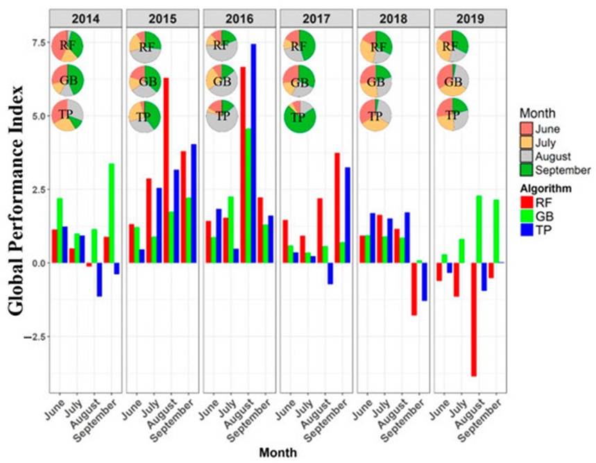
Figure 4. Annual trends and monthly fluctuations of the Global Performance Index (GPI) values.
Global interpretability through SHAP values maps out the explicit contributions of individual environmental predictors to the target variable. The underlying architectures utilize baseline regression frameworks integrated with a tree-based explainer to derive these SHAP values. Following the test set results from July 2019 and August 2019—which yielded mean accuracy metrics of 0.35 for RF and 0.68 for GB—a targeted evaluation explored the dependencies between environmental features and PM2.5 concentrations. The assessments showed that RH in July 2019 and UWIND in August 2019 represented the primary drivers for forecasting PM2.5 across both the RF and GB configurations. In the southern region specifically, both regression models yielded prominent positive SHAP scores above 0.6 for UWIND within the August 2019 dataset, accounting for nearly 66.30% of the total variance.
Furthermore, because Aerosol Optical Depth (AOD) is closely linked to PM2.5 behavior, the interactions between AOD and its governing features were evaluated. Ambient temperatures above 300 K, RH levels spanning ~76 to 78, and a UWIND velocity near −1.0 m/s were the most critical drivers for both RF and GB models during July and August of 2019.
Because fine particulate matter PM2.5 is a critical atmospheric threat, mapping its fluctuations helps uncover the mechanisms governing its distribution, providing essential data for environmental policy design. The SHAP approach was applied to clarify feature importance for the optimal pipeline results generated by the automated TP model during PM2.5 estimation. These SHAP metrics determine the precise weight each variable exerts on the final output, and Figure 5 illustrates the distribution of these values alongside overall feature rankings. Beeswarm visualizations display the continuous distribution of variables across distinct categories alongside their SHAP values, clarifying data density, underlying patterns, or anomalies within specific groups. Due to data gaps, the Normalized Difference Vegetation Index (NDVI)—which evaluates live green canopy via satellite observations—showed low importance across all time blocks. This implies that the model is less sensitive to changes in vegetative cover than it is to atmospheric trends or human-driven activities.
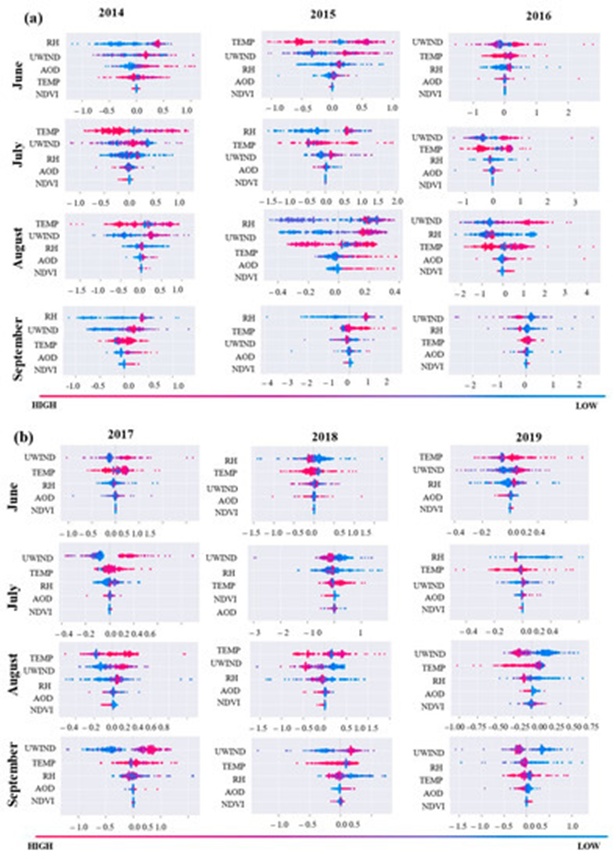
Figure 5. SHAP value distributions for the RF Tree Explainer visualized via beeswarm plots across feature importance tiers: (a) June–September for the 2014–2016 timeframe, and (b) June–September for the 2017–2019 timeframe. The gradient color scheme shifting from red to blue maps the model's output values from high to low.
The zonal wind velocity component, UWIND (which captures east–west wind vectors), achieved the highest mean SHAP value in 2016, establishing it as the primary predictive feature for determining PM2.5 concentrations during that annual cycle. This prominence is likely attributable to localized atmospheric circulation patterns or other dominant environmental drivers unique to 2016. Conversely, relative humidity (RH, representing the atmospheric water vapor content relative to saturation) emerged as a critical feature across nearly all months of 2015, with the exception of June. This variation may stem from fluctuating meteorological configurations or alternative environmental inputs modifying regional moisture profiles during that specific year.
The mean SHAP value plot presented in Figure 6 illustrates a method for consolidating SHAP measurements across all observations to compute the aggregate influence of each variable on the system's output. The accompanying histogram portrays the importance distribution of categorical features, organized from maximum to minimum impact. According to the bar chart, UWIND exhibited the maximum mean SHAP value relative to all other variables, confirming its status as the most critical overall determinant for forecasting PM2.5 levels. This pattern might be explained by a robust correlation between UWIND and other critical predictive features within the model architecture, or because it captures fundamental characteristics of atmospheric stability and air quality that the model is tasked with predicting. Collectively, these observations clarify the underlying mechanisms driving PM2.5 variability and underscore the necessity of integrating diverse environmental metrics when simulating particulate concentrations.
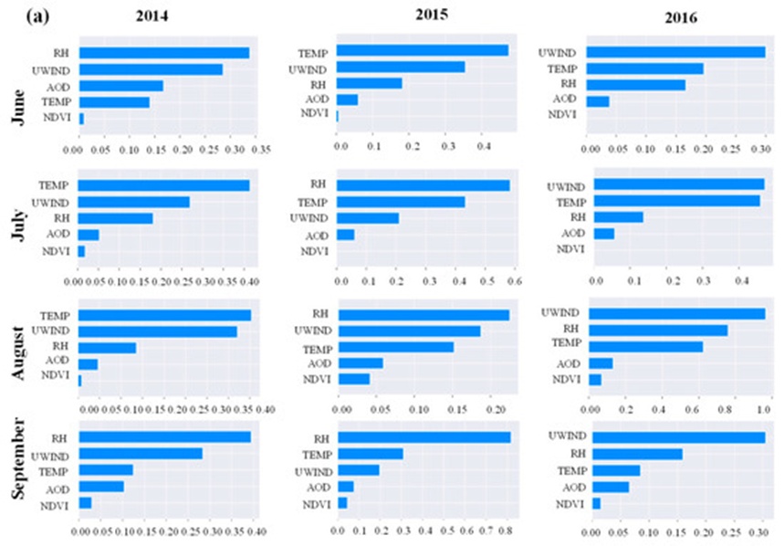
Figure 6. Aggregate distribution of SHAP values for the RF Tree-based explainer stratified by feature importance tiers: (a) June–September for the 2014–2016 interval, and (b) June–September for the 2017–2019 interval. The graphic maps the distribution of feature importance metrics in a high-to-low hierarchical sequence.
The global interpretation is illustrated via the heatmap visualizations in Figures 7a and 7b. These heatmaps serve to depict the linearized density and continuous distribution of the dataset, with numerical values mapped onto colored lines. During August 2016, UWIND exhibited the maximum feature importance, corresponding to the highest MAE and MAPE metrics derived from the XGB regression framework. In contrast, RH emerged as the dominant feature in Figure 5, matching the lowest MAPE metric yielded by the XGB regressor in July 2019. Figure 7 demonstrates that the inclusion of the RH variable in July 2019 enhanced the predictive accuracy for over 150 individual observations, accounting for an explanatory contribution exceeding 37% with SHAP values of 0.2. Ambient temperature registered as the second most influential factor (5–6%), with SHAP values ranging between 20 and 25. The remaining environmental features generated negligible impacts, with SHAP values hovering near 0. Consequently, the SHAP value distributions and global heatmap explanations clarify the inner workings of the model and underscore the varying importance of specific features when forecasting PM2.5 levels. The investigation confirms that UWIND was the primary predictive driver in August 2016, whereas RH assumed the most prominent role in July 2019.
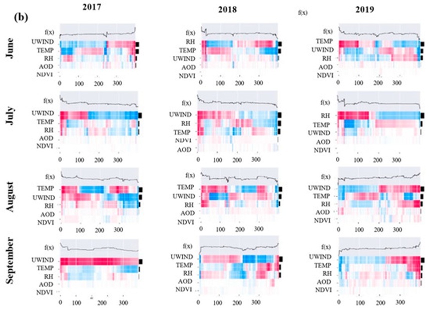
Figure 7. Paired heatmap visualizations representing distinct temporal windows: (a) June–September (2014–2016) and (b) June–September (2017–2019). The diagrams illustrate SHAP value distributions for the RF Tree-based explainer and relative feature importance using a color gradient from high to low impact; the model output is presented along the upper x-axis in log odds, the y-axis ranks features by their relative importance, and observations are grouped via functional clustering.
The research also assessed various explanation metrics applied to RF, GB, and XGBoost architectures using the datasets from July and August 2019. The Random explainer produced larger explanation errors across all tree-based regression frameworks, though its performance improved when positive model outputs were omitted . Conversely, the Partition, Permutation Part, Tree, Exact, and Permutation explainers minimized error rates when clarifying the RF model. Furthermore, the Tree, Partition, and Permutation Part explainers yielded fewer explanation errors when evaluated against the July and August 2019 data.
The spatio-temporal variations in PM2.5 estimated by the RF and GF algorithms are visualized in Figure 8. High and low concentrations of PM2.5 are quantified in \mu\text{g m}^{-3}. To analyze these spatial and temporal dynamics, unoptimized algorithms were selected based on achieving the peak performance score on the GPI. August 2016 displayed elevated concentrations under the RF model relative to the other time periods examined. According to the monthly spatial variations projected by the RF model, the maximum spatial density variation was concentrated within central Singapore. Compared to alternative months in 2016, August exhibited the most pronounced fluctuations in PM2.5 loading, with elevated concentrations in the northern territory and the lowest values localized in eastern Singapore. XAI diagnostics revealed that UWIND exerted a dominant control among all variables across the entirety of 2016; furthermore, RH and TEMP also provided substantial predictive contributions, though their variance intensities differed.
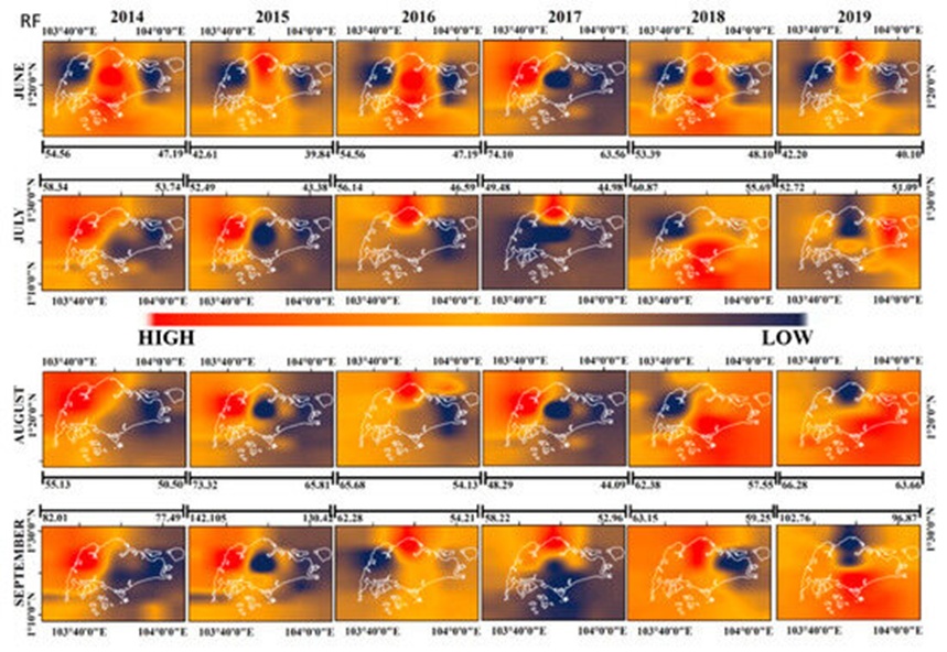
Figure 8. Spatial mapping of PM2.5 concentration forecasts generated via RF regression for the June–September intervals spanning 2014 to 2019.
By comparison, Chen et al. [67] determined that overall R^2 values hovered around 0.88 when utilizing an RF architecture across various sites in China, while Hu et al. [68] noted that daily PM2.5 fluctuations modeled via RF techniques achieved R^2 scores of 0.80 within the United States. In this study centered on Singapore, the aggregate temporal mean R^2 values reached approximately 0.65. The divergence among these statistical values is likely attributable to highly dynamic shifts in local meteorological variables and topographic layouts.
To provide a transparent overview of how machine learning models shift their predictions regarding PM2.5 concentrations, several core themes are emphasized below:
Machine Learning Algorithm Architecture: The underlying structural design of the machine learning models (RF, GB, and TP) directly dictates the internal prediction mechanisms and the resulting spatial estimations. For example, as an ensemble technique, RF aggregates outputs from multiple independent decision trees; GB sequentially constructs an ensemble of decision trees where each subsequent model minimizes the residuals of its predecessor; TP functions as an evolutionary optimization algorithm tailored for hyperparameter refinement and model/feature selection. These frameworks are capable of capturing highly intricate interactions within the datasets.
Incorporation of External Explanatory Features: Variables such as NDVI, temperature, wind velocity, and humidity directly govern the dispersion, chemical transformation, and localized pooling of particulate matter in the lower atmosphere. Consequently, these inputs provide substantial explanatory power regarding the spatial and temporal dynamics of PM concentrations.
Necessity of Spatio-Temporal Modeling and Data-Driven Inference: Optimal machine learning configurations offer clear insights into how effectively PM2.5 concentrations are mapped across different geographic locations within the study zone. Implementing time-series and spatial forecasting helps untangle the cyclical, monthly characteristics of PM2.5 variations while factoring in the compounding effects of weather variables.
In the XAI interpretability workflows applied to the RF model, fluctuations in meteorological inputs like UWIND and RH strongly governed the PM2.5 predictions, a result of dynamic weather shifts and seasonal modifications [69]. When examining annual fluctuations, the models displayed considerable variance in their overall GPI scores, particularly across the 2014, 2015, 2016, 2017, and 2018 cycles.
Among the various machine learning explainers tested, tree-based explainers delivered superior predictive diagnostics, demonstrating that tree-structured architectures are highly effective at simulating PM2.5 dynamics. These tree models maintained elevated predictive accuracy even when confronted with missing spatial pixel data across random locations. Nevertheless, the spatial and temporal resolutions of the available datasets pose a clear limitation that can impact the precision of the final outputs. Despite this constraint, the analytical framework developed here offers valuable decision-support tools for environmental policy and air quality management. For context, Ji et al. [34] leveraged RF models to evaluate how various air pollutants, including PM2.5, affected pediatric respiratory disease rates in Taizhou, China; RF emerged as the top-performing framework in [34], matching the conclusions of this study. Additionally, Gu et al. [33] deployed a hybrid model merging an interpretable architecture with a deep neural network, yielding an overall RMSE of 15.0835. Bai et al. [70] utilized an LSTM framework to achieve RMSE values between 13 and 14 for PM2.5 modeling in China; in comparison, the predictions in this study achieved an RMSE of 0.49 for RF and 0.77 for TP, representing the top metrics among the time-series models evaluated.
Analyzing PM2.5 variations through regression frameworks and XAI techniques has clarified critical predictive features and their relative roles in modeling particulate concentrations. The combination of SHAP value distributions and global explanations provides a robust methodology for mapping PM2.5 levels while ensuring the interpretability and transparency of atmospheric models. Evaluating feature contributions highlights the critical need for comprehensive, adaptive frameworks in air quality modeling. In this research, different variables assumed primary importance across different timeframes to optimize PM2.5 predictions. Although these simulations are subject to data gaps and structural uncertainties (such as sensor noise and coarse resolutions), the feature contribution analysis proved highly robust and logically sound under direct verification. The Tree explainer demonstrated superior performance compared to alternative SHAP explainers when applied to RF, GB, and XGBoost models. Furthermore, the RF model significantly outperformed the GB model regarding both MAE and MAPE metrics.
When comparing the unoptimized baselines of RF and GB, the RF model demonstrated strong capabilities in predicting PM2.5 concentrations, whereas the GB model tended to produce overestimated predictions. Following hyperparameter tuning of the XGB regressor and an optimization process using the TP model's genetic iterations, the PM2.5 concentrations for July 2019 were modeled with higher accuracy relative to other periods based on a joint evaluation of MSE, RMSE, MAE, and MAPE. These outcomes suggest that the XGBoost regression architecture is a highly effective tool for simulating PM2.5 loading, yielding minimized MAE and MAPE scores compared to alternative frameworks, with RH acting as a critical parameter for enhancing model accuracy. Global SHAP analysis shed light on the relative weight of input features for both the RF and GB frameworks; UWIND emerged as the definitive driver for PM2.5 tracking in August 2016, whereas RH took precedence in July 2019. This shift demonstrates that feature importance varies across distinct seasons and environmental settings, underscoring the model's sensitivity to micro-climatic dependencies. Ultimately, regression models coupled with XAI tools are vital for forecasting and diagnosing PM2.5 distributions, offering crucial analytical support for regulatory frameworks and air quality management strategies.
The authors would like to acknowledge the National Institute of Technology Rourkela for providing lab facilities. The authors are thankful to Yuming Guo, Monash University, for his valuable suggestions and stimulating scientific discussions. We are also thankful to the National Environmental Agency, Singapore, for providing the in situ observations of PM2.5 over Singapore.
None
None
None
Open Access The author(s) retain copyright. This article is licensed under the Creative Commons Attribution-NonCommercial-ShareAlike 4.0 International License. It may be shared and adapted for non-commercial purposes with appropriate attribution, an indication of changes, and distribution of adaptations under the same license. Third-party material may be subject to separate terms identified in its credit line. View the license at https://creativecommons.org/licenses/by-nc-sa/4.0/.
 Transparent Intelligence Publishing