A multitude of studies demonstrate that robust predictive models for identifying microorganisms can be successfully developed by combining Raman micro-spectroscopy with chemometric techniques, frequently yielding highly accurate outcomes. Progress in machine learning alongside increased software availability has simplified the process for researchers to construct predictive frameworks from intricate data arrays. Conversely, the underlying reasons for the high accuracy of these classifications remain under-investigated. This study analyzes Raman spectroscopic datasets from fungal spores and carotenoid-producing microorganisms to demonstrate that successful differentiation is frequently independent of peak positions or subtle variations in spectral band ratios caused by minor biochemical differences among the organisms. Instead, distinctive baseline variations in biochemically related microorganisms, which may be amplified by specific data preprocessing routines, play a critical role; furthermore, seemingly neutral spectral intervals can significantly influence a convolutional neural network. By applying a technique known as Gradient-weighted Class Activation Mapping, we investigate the internal mechanics of convolutional neural networks within microbiological domains to determine the precise Raman spectral bands driving successful classification.
The rapid and precise identification of microorganisms is crucial across multiple domains, including medical diagnostics for timely and appropriate patient intervention, and food processing to guarantee consumer safety. Conventional approaches for distinguishing microbial species frequently depend on cultivation, which invariably demands substantial time and resource expenditure. Accelerated alternatives exist, including DNA-targeted assays and matrix-assisted laser desorption ionization-time of flight mass spectrometry (MALDI-TOF MS). Techniques utilizing optical molecular spectroscopy, particularly Raman spectroscopy, offer another viable avenue for microbial differentiation [1]. This strategy requires compiling a reference library of representative Raman spectra to train mathematical models capable of classifying newly acquired, unknown profiles. A significant body of research has verified that reliable predictive frameworks for microorganisms can be constructed using Raman micro-spectroscopy integrated with chemometrics, often achieving outstanding accuracy [1-4].
Individual bacterial cells can even be resolved via surface-enhanced Raman microscopy or specialized metallic substrates [5-7], potentially removing the need for time-intensive pre-enrichment and culture phases. In prior investigations, we employed Raman microscopy to formulate predictive frameworks for identifying distinct isolates and species of fungal spores [8] and for distinguishing among 21 species of bacteria and yeasts [9]. These efforts yielded highly precise classifications, with accuracies exceeding 98% when utilizing support vector machines (SVM). The evolution of machine learning techniques and the proliferation of open-source software have made the generation of dependable predictive models from complex datasets increasingly accessible to non-specialists.
When these analytical strategies are deployed outside the core domain of machine learning research, the underlying mechanisms enabling such high model accuracy are frequently left unexamined. A study by Kanno et al. partially explores this area by applying random forest machine learning to highlight the primary features within a Raman spectrum-based model used for microbial classification [10]. Minor variations in the biochemical makeup of microorganisms generate distinct Raman spectral signatures, which enables differentiation [1, 11] provided that data volume and quality are sufficient. Multiple environmental and experimental variables can affect a Raman spectrum; however, most of these can be managed by standardizing measurement conditions. External factors influencing the Raman spectra of microorganisms, such as the formulation of the growth medium [12, 13] or the duration of incubation [14], are easily controlled. Yet, even with thorough standardization, mathematical preprocessing of the spectral data remains not only recommended but often vital for cultivating high-performing predictive models [15].
Variations in the baseline, typically introduced by confounding fluorescence, or fluctuations in the absolute intensity of a Raman spectrum, can be mitigated through baseline correction and normalization techniques. Similarly, smoothing algorithms can prevent random noise from being misidentified as a meaningful classification feature. Predictive workflows can be further optimized by decreasing data dimensionality via principal component analysis (PCA), which filters out redundant or disruptive spectral features that might otherwise compromise classification performance [16].
In the present study, we evaluate whether microbial differentiation is genuinely dictated by subtle shifts in Raman spectral bands or if entirely separate phenomena are responsible. To explore this, we trained convolutional neural network (CNN) models using two datasets obtained from earlier reports [8, 9]. The first dataset comprises Raman spectra from fungal spores, exhibiting exceptionally high spectral similarity across certain isolates and species [8]. The second dataset consists of specific microorganisms characterized by carotenoid pigments, which serve as highly effective diagnostic markers [9, 17].
Although deep learning architectures have driven artificial intelligence (AI) to unprecedented capabilities, the interpretability and transparency of these models remain an active area of scientific inquiry [18, 19]. Among the most prominent strategies for visually decoding classification decisions in CNNs is Gradient-weighted Class Activation Mapping (Grad-CAM) [20, 21]. Grad-CAM isolates the influential neurons within a model relative to a given classification task, offering a visual explanation of "where" the network concentrates its attention during prediction. Grad-CAM is adaptable to diverse convolutional network structures; in this study, we apply it to reveal the specific segments of Raman spectra that are most critical to the classification process by treating each spectrum as a one-dimensional image.
The experimental protocols for cultivating and isolating fungal spores are detailed in the 2021 study by Hetjens et al. [8]. The specific cultivation conditions for the microorganisms are described in the March 2022 report by Tewes et al. [9]. The nomenclature, corresponding abbreviations, and the total number of collected Raman spectra for each investigated species are summarized in Table 1.
Table 1. All used fungal spores and carotenoid-containing microorganisms.
Microorganism | Abbreviation | Number of Spectra | |
Fungal spores | Metarhizium brunneum Cb16III | Cb16III | 642 |
Metarhizium brunneum Ca8II | Ca8II | 562 | |
Metarhizium brunneum Cb15III | Cb15III | 525 | |
Metarhizium pemphigi X1c | Mpemp | 847 | |
Beauveria bassiana | Bbass | 372 | |
Carotenoid- | Chryseobacterium indolgenes | Cin | 684 |
Kocuria rosea | Kro | 639 | |
Micrococcus luteus | Mlu | 1842 | |
Staphylococcus aureus | Sau | 1094 | |
Xanthophyllomyces dendrorhous | Xde | 658 |
The conidia and bacterial suspensions were deposited under sterile conditions onto a $\text{SiO}_2$-coated silver mirror substrate (PFR14-P02, Thorlabs, Lübeck, Germany). This silver substrate was positioned on the automated stage of the Raman instrument. Microscopic examination (100× magnification) was used to locate target regions containing spores or carotenoid-bearing microorganisms. Prior to evaluating subsequent samples, the substrate surface was cleaned using an acetone-soaked cotton pad, followed by an ethanol wash with a lint-free task wiper, and a final rinse with sterile deionized water. Comprehensive breakdowns of the sample preparation steps are available in references [8] (for fungal spores) and [9] (for carotenoid-containing microorganisms).
Spectral collection was performed using a confocal Raman microscope (inVia Renishaw, Gloucestershire, UK) configured with a 633 nm excitation laser line and a 100× objective lens (numerical aperture of 0.85). Conidia samples were interrogated using a 1.5 s integration time at an incident laser power of approximately 0.7 mW at the sample surface (focused spot diameter of roughly 5 µm), with 15 co-additions recorded per spectrum. All carotenoid-containing microorganisms were examined with an integration time of 1.5 s and a laser power of approximately 3.5 mW at the sample (focused spot diameter of roughly 7.5 µm). The system provided a spectral resolution of approximately 1.1 wavenumbers. Fully detailed accounts of the spectral acquisition configurations can be found in publications [8] (fungal spores) and [9] (carotenoid-containing microorganisms).
Computational processing of the raw data was carried out within the MATLAB R2021b environment (MathWorks, Natick, MA, USA). Following numerical interpolation of the collected spectra, a low-pass filter (LPF) was implemented to handle baseline deviations and smooth the signals. Standardized scaling was then applied across all spectral data using z-score normalization. To explore initial distribution trends and evaluate how easily the samples could be categorized, the data underwent a PCA. However, the subsequent deep learning workflows bypassed these principal components (PCs) entirely, utilizing the comprehensive, fully preprocessed spectral vectors instead. For both the fungal conidia and the carotenoid-bearing microbes, independent network architectures were developed. To verify that random initialization variations did not arbitrarily alter the spectral domains flagged as crucial by the networks (subsequently audited via Grad-CAM), two separate iterations of each model were trained using identical hyper-parameters but distinct random weight initialization seeds.
The classification networks were engineered via TensorFlow version 2.6.2 and feature a sequential arrangement of three convolutional layers, with each layer deploying 16 filters alongside a kernel width of five. Every convolutional block integrates batch normalization, a rectified linear unit (ReLU) activation function, and a subsequent max pooling stage. Downstream from a global average pooling operation, the data passes through a dense layer containing 256 nodes configured with ReLU activations and a 0.3 dropout probability, ultimately terminating in a 5-dimensional output layer regulated by a softmax activation function. This configuration yields a total of 8421 adjusting parameters. Network optimization was driven by the Adam algorithm at a fixed learning rate of 0.0001, minimizing a Sparse Categorical Cross-Entropy loss function over 1500 training epochs with a mini-batch size of 64.
Grad-CAM was deployed to extract localized activation intensity maps corresponding to accurate target classifications. Because the Grad-CAM algorithm calculates integrated gradients relative to the final convolutional layer, it yields a 256-point heatmap that was subsequently upscaled to match the original input dimension using the bilinear interpolation library within OpenCV [22]. To isolate class-specific trends, individual activation topographies were aggregated into a mean class activation map, filtering exclusively for instances where the underlying prediction matched the ground truth.
Because raw Raman signals are prone to external experimental variances unrelated to the native biochemical traits of different strains, structured data preprocessing represents a vital phase in microbial taxonomy [23, 24]. For this reason, modeling efforts involving raw, unconditioned datasets were intentionally excluded from this study.
The gathered spectral curves for the fungal spores are presented in Figure 1. Exceptionally high degrees of overlapping spectral features are visible when comparing Cb16III against Cb15, as well as Ca8II against Mpemp. The broad variance observed within the Bbass sample cohort was primarily driven by strong background fluorescence interference. Distinct boundary artifacts are visible at the outer edges of the conditioned spectra (Figure 1b) due to the constraints of the applied LPF; the filter introduces a sharp downward pull near 600 cm−1 and creates a noticeable inflection point near 1675 cm−1.
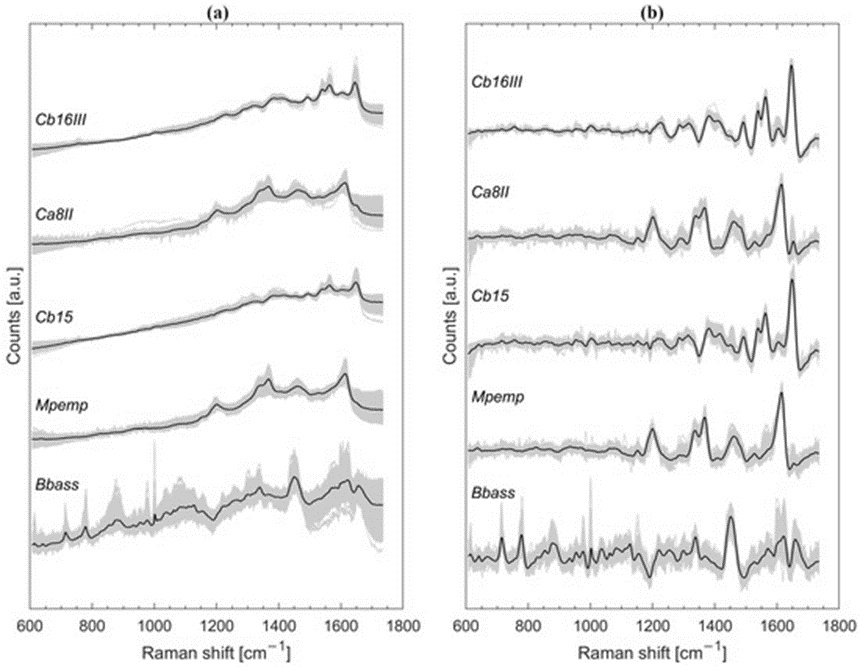
Figure 1. Graph depicting the complete spectral collection for the fungal conidia (represented by grey lines) overlaid with the calculated mathematical mean for each group (distinguished by black lines and separated vertically along the intensity axis). The visual data compares the raw, z-score-scaled spectral curves (a) against the fully preprocessed outputs that underwent baseline correction, smoothing, and standardized scaling (b).
Prior to conditioning, the raw Raman signatures of the carotenoid-bearing microbes (Figure 2a) display their widest data dispersion within the 600 to 1000 wavenumber region, an effect that stands out clearly in the Cin and Sau groups. This baseline scattering is sharply constrained following the preprocessing steps (Figure 2b). The two dominant spectral bands emerging near 1150 and 1525 cm−1 across all traces in Figure 2 originate from native carotenoid pigments [17]. These prominent bands display distinct, minor horizontal shifts across different species, an attribute that strongly supports straightforward class separation. Slight negative slants are also visible in the processed curves (Figure 2b) flanking the intense signal peak at roughly 1525 cm−1. Furthermore, Sau and Xde exhibit a rapid drop in intensity immediately following the second major peak near 1150 cm−1.
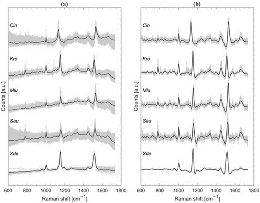
Figure 2. Comprehensive plotting of the carotenoid-producing microbial Raman profiles shown in grey, with the calculated average spectrum for each target group highlighted in black bold lines (offset along the vertical axis for visual separation). The panels provide a comparison between the unconditioned, normalized data arrays (a) and the preprocessed spectral configurations following baseline flattening, filtering, and z-score transformation (b).
It is worth noting that the specific PCs capturing the highest levels of data variance do not automatically function as the most effective features for classification models [25]. In certain scenarios, lower-order PCs can provide superior discriminatory insight compared to high-variance components. Even so, PCA remains an uncomplicated and dependable technique for exposing latent structures within high-dimensional datasets [26].
As illustrated in the three-dimensional space of Figure 3a, the first three PCs struggle to establish clear spatial boundaries between Cb16III and Cb15. Similarly, the data envelopes for Ca8II and Mpemp show noticeable intermixing. In contrast, Bbass segregates cleanly from the rest of the sample distribution, showing strong isolation. Matching the initial observations of carotenoid-related bands in Figure 2b, the microbial samples split into isolated, well-defined clusters when mapped against the first three coordinates of the PCA space (Figure 3b).
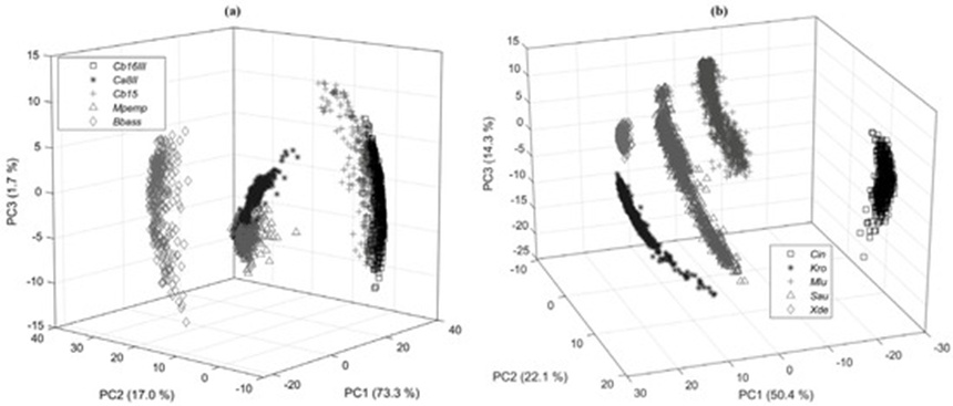
Figure 3. > Three-dimensional scatter plots mapping the initial three principal coordinates derived from the preprocessed Raman data matrix for the fungal conidia isolates (a) and the carotenoid-pigmented bacterial strains (b).
To validate the performance of the convolutional models, a 5-fold cross-validation scheme was implemented, setting aside a 20% holdout fraction for test evaluation. To prevent overfitting, a 15% partition of the active training pool served as an internal validation set to identify and preserve the peak-performing model state. This preserved network was subsequently benchmarked against the isolated test dataset. The resulting mean precision, recall, F1-score, and support values for the initial fungal conidia network (model 1) are compiled in Table 2. Precision values for Cb16III (0.98), Cb15 (0.96), and Bbass (1.0) indicate exceptional accuracy. While model 1 showed marginally lower precision when classifying Mpemp (0.89) and Ca8II (0.88), the overall rate of correct identification hovered near 90%. The secondary replication model (model 2), leveraging an identical layer setup, yielded very similar classification metrics (Table 3). Serious deviations between these two models would normally point to a weak or insufficient data volume, which is clearly not the case here.
Table 2. Precision, recall, F1 score and support with model 1 for fungal spores.
Microorganism | Support | F1-Score | Recall | Precision |
Cb16III | 131 | 0.97 | 0.97 | 0.98 |
Ca8II | 133 | 0.86 | 0.83 | 0.88 |
Cb15 | 105 | 0.96 | 0.97 | 0.96 |
Mpemp | 181 | 0.90 | 0.92 | 0.89 |
Bbass | 74 | 0.99 | 1.00 | 1.00 |
accuracy | 624 | 0.93 |
| |
macro avg | 624 | 0.94 | 0.93 | 0.94 |
weighted avg | 624 | 0.93 | 0.93 | 0.93 |
Table 3. Precision, recall, F1 score and support with model 2 for fungal spores.
Microorganism | Support | F1-Score | Recall | Precision |
Cb16III | 131 | 0.98 | 0.98 | 0.97 |
Ca8II | 133 | 0.85 | 0.82 | 0.90 |
Cb15 | 105 | 0.97 | 0.97 | 0.98 |
Mpemp | 181 | 0.90 | 0.93 | 0.87 |
Bbass | 74 | 0.99 | 1.00 | 1.00 |
accuracy | 624 | 0.93 |
| |
macro avg | 624 | 0.94 | 0.94 | 0.94 |
weighted avg | 624 | 0.93 | 0.93 | 0.93 |
The classification parameters generated by both the primary network (Table 4) and the secondary network (Table 5) for the carotenoid-bearing microbes reached a uniform score of 1.0 across all categories, indicating absolute accuracy in identifying every tested species.
Table 4. Precision, recall, F1 score and support with model 1 for carotenoid-containing microorganisms.
Microorganism | Support | F1-Score | Recall | Precision |
Cin | 137 | 1.00 | 1.00 | 1.00 |
Kro | 128 | 1.00 | 1.00 | 1.00 |
Mlu | 368 | 1.00 | 1.00 | 1.00 |
Sau | 219 | 1.00 | 1.00 | 1.00 |
Xde | 130 | 1.00 | 1.00 | 1.00 |
accuracy | 983 | 1.00 |
| |
macro avg | 983 | 1.00 | 1.00 | 1.00 |
weighted avg | 983 | 1.00 | 1.00 | 1.00 |
Table 5. Precision, recall, F1 score and support with model 2 for carotenoid-containing microorganisms.
Microorganism | Support | F1-Score | Recall | Precision |
Cin | 137 | 1.00 | 1.00 | 1.00 |
Kro | 128 | 1.00 | 1.00 | 1.00 |
Mlu | 368 | 1.00 | 1.00 | 1.00 |
Sau | 219 | 1.00 | 1.00 | 1.00 |
Xde | 130 | 1.00 | 1.00 | 1.00 |
accuracy | 983 | 1.00 |
| |
macro avg | 983 | 1.00 | 1.00 | 1.00 |
weighted avg | 983 | 1.00 | 1.00 | 1.00 |
The Grad-CAM maps were established by averaging the mathematical activations recorded across all true-positive classification events and scaling the final output values between 0 and 1. The average spectral trace and the associated variance envelope for each distinct strain are plotted as a solid line and a shaded region, respectively. These activation metrics are mapped directly over the spectral lines as vertical heat bands. A deeper color tone within a specific band highlights a wavenumber region that the network heavily weighted during its classification decision (using the reference scale adjacent to each visualization in Figures 4 and 5). Because these plots show the cumulative average across all successfully categorized profiles within a specific class, they highlight which spectral zones dictate the model's general success; however, this combined view does not indicate that every individual sample concurrently activates all highlighted regions.
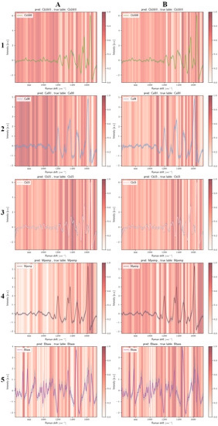
Figure 4. Average Raman curves for the fungal conidia isolates Cb16III (A1), Ca8II (A2), Cb15 (A3), Mpemp (A4), and Bbass (A5) superimposed with the normalized Grad-CAM diagnostic heat fields reflecting the decision-making pathways of model 1. Panels (B1) through (B5) display the corresponding mean Raman signals for the same conidia groups mapped with the normalized Grad-CAM importance indicators for model 2. The vertical axes reflect z-score standardized spectral intensity values, while the Grad-CAM importance metrics are scaled continuously from 0 to 1, moving from white to saturated dark red.
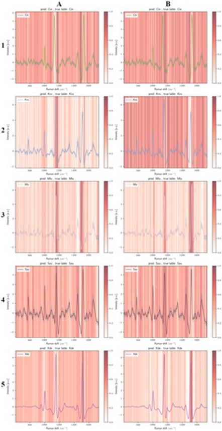
Figure 5. Mean Raman traces for the carotenoid-bearing microbial targets Cin (A1), Kro (A2), Mlu (A3), Sau (A4), and Xde (A5) paired with the normalized Grad-CAM activation signatures extracted from model 1. Panels (B1) through (B5) present the identical target species mean profiles paired with the normalized Grad-CAM weight distributions extracted from model 2. Standardized z-score values define the vertical axes, and the Grad-CAM attention gradient is mapped linearly from zero up to one (progressing from white to dark red).
The calculated average spectral tracks for each fungal conidia category, alongside the specific spectral zones leveraged by the deep learning networks for classification, are presented in Figure 4(A1–5,B1–5). For the isolate Cb16III (Figure 4(A1)), the classification framework heavily recruits numerous intervals within the lower wavenumber domain (approximately 600–1200 cm−1). This particular spectral region is characterized by relatively low-intensity signals, and the moderately more distinct bands near 753 and 1001 cm−1 are actually assigned lower significance by model 1. Similarly, the more prominent profiles located between 1200 and 1565 cm−1 are less utilized, with Grad-CAM predominantly highlighting the peripheral boundaries flanking these main bands. Consequently, within model 1 for Cb16III (Figure 4(A1)), the positions at 1464 cm−1 and 1668 cm−1 emerge as highly critical for the categorization process, despite lacking explicit peak maxima. The domains highlighted by Grad-CAM in the secondary network configuration (Figure 4(B1)) show reasonable alignment with model 1, though the lower wavenumber span (600 to 1200 cm−1) is allocated slightly less weight. The solitary prominent peak of Cb16III flagged in deep red by Grad-CAM within model 2 is the sharp sub-peak located at 1538 cm−1.
The marked Grad-CAM zones in model 1 for the conidia isolate Cb15 (Figure 4(A3))—which shares an extremely close Raman spectroscopic profile with Cb16III—appear nearly inverted relative to Cb16III (Figure 4(A1)). Here, the lower wavenumber range receives minimal attention, with the notable exceptions of the signatures near 753 and 1001 cm−1 (Figure 4(A3)). Furthermore, in an exactly opposing manner, model 1 entirely bypasses the intervals immediately preceding and following the dominant peak near 1649 cm−1, whereas these identical zones are highly prioritized in Cb16III. The Grad-CAM highlighted bands for Cb15 in model 1 (Figure 4(A3)) display variations when compared to model 2 for Cb15 (Figure 4(B3)); specifically, model 1 flags the precise valley separating the doublet peak at 1383 and 1413 cm−1 in deep red, whereas model 2 focuses directly on the actual peak maxima rather than the intermediate interval. A noticeable feature for Cb15 across both model iterations is the strong Grad-CAM activation in the region exceeding 1647 cm−1, a phenomenon primarily induced by the deployed baseline filtration method (visualized by comparison with the unconditioned Cb15 spectrum in Figure 1a). It is highly probable that minor discrepancies in background fluorescence are amplified following data preprocessing, thereby creating artificially enhanced classification features. Naturally, it must be acknowledged that the deployment of alternative baseline removal techniques would likely shift the network's focus toward completely different spectral zones. Preliminary evaluations into this behavior indicate that even baseline filters optimized for higher performance still yield networks that depend on seemingly non-specific spectral regions for group differentiation.
Members of the Metarhizium genus generate native colored pigments, akin to the carotenoid-producing microorganisms. The Raman profiles of Metarhizium display diagnostic bands around 1380–1400 cm−1 and 1580–1600 cm−1, suggesting that both conidia types likely synthesize melanin [27]. Because the specific pigment characteristics do not vary among the evaluated Metarhizium fungal isolates within this spectroscopic dataset, alternative spectral fluctuations must drive the successful classification. Initial comparison of the unconditioned profiles in Figure 1a for Cb16III and Cb15 reveals that while the curves are remarkably similar, the absolute peak definition is generally more muted for Cb15. Following mathematical data conditioning, this distinction becomes nearly imperceptible (Figure 1b).
A comparable divergence in network behavior is observed between Ca8II and Mpemp when analyzing model 1 (Figure 4(A2,4)) and model 2 (Figure 4(B2,4)). For this pair, it is especially evident that models 1 and 2 exploit completely disparate spectral intervals, despite utilizing identical architectural configurations and training parameters. For Mpemp, the spectral zones situated above 1640 cm−1 are highly prioritized by the CNN across both training runs, even though no authentic spectral features exist there; instead, this zone contains a structural distortion artifact introduced by the baseline filter (verified by comparing Mpemp from Figure 4 against the raw/conditioned Mpemp traces in Figure 1).
The Raman signatures of Bbass diverge dramatically from the remaining fungal spore categories. Rather than isolating a small number of prominent spectral landmarks, the network considers an expansive array of features; these include the peaks at 714 cm−1, 744 cm−1, the phenylalanine (Phe) band at 1003 cm−1 (most notably in model 1), and the broader band at 1450 cm−1. Although differences exist between the Grad-CAM maps of Bbass generated by model 1 and model 2, these variations are far less pronounced than those seen in Mpemp, which represents a much more challenging target for differentiation due to its extreme spectral convergence with Ca8II. Given that Bbass conidia are highly distinct from the other species via Raman spectroscopy, it might intuitively be assumed that a minimal set of unique features would suffice for identification. However, Figure 4(A5,B5) clearly illustrates that a wide variety of signals recruit network attention. Thus, the CNN operates in a manner entirely counter to this logical assumption. In future investigations, it would be highly instructive to isolate training exclusively to a two-species model to track loss dynamics and Grad-CAM outputs, thereby concretizing this observation.
The intense bands at approximately 1133 and 1530 cm−1 arising from native carotenoids in Cin are largely ignored by the CNN in both model 1 (Figure 5(A1)) and model 2 (Figure 5(B1)). Instead, the negative slope dropping near 1504 cm−1, along with the relatively featureless baseline zone around 1176 cm−1, holds major significance for the network's classification decisions.
A particularly striking finding emerges when comparing the Grad-CAM maps for Kro (Figure 5(A2,B2)), which display almost perfectly inverted attention profiles. In model 1, network attention is concentrated almost exclusively on the peak around 1154 cm−1, its immediate rightward tail, and the brief negative slope near 1538 cm−1, while all remaining spectral intervals are treated as statistically negligible (Figure 5(A2)). Conversely, in model 2, nearly every spectral region is deemed highly significant by the CNN, save for the primary carotenoid band located near 1513 cm−1.
The Grad-CAM highlights for Mlu (Figure 5(A3,B3)) indicate that the network focuses intensely on the boundaries flanking the main carotenoid peaks; specifically, in model 1 (Figure 5(A3)), the zone directly preceding the 1528 cm−1 peak is highly prioritized. A narrow spectral window immediately following the peak at >1003 cm−1 also recruits attention during Mlu classification, whereas the peak itself—which is attributed to phenylalanine (Phe) [28]—proves far less critical to the CNN.
For Sau, both model iterations generate highly distributed Grad-CAM activation patterns across multiple spectral domains (Figure 5(A4,B4)). Model 1 is characterized by a complete omission of the negative slope near 1496 cm−1, whereas model 2 entirely bypasses the area following the Phe peak at roughly 1003 cm−1 (Figure 5(B4)). In a complementary fashion, the peak near 781 cm−1—which is linked to phosphate bonds, cytosine, uracil, or thymine [7, 29]—exhibits low importance in model 2 (Figure 5(B4)) but is heavily emphasized in model 1 (Figure 5(A4)). Crucially, however, the primary diagnostic features driving the classification of Sau remain the carotenoid-associated signals around 1158 cm−1.
Although the highly compact spatial clustering of Xde within the PCA plot (Figure 3b) implies an effortless separation, model 1 recruits an extensive array of spectral regions to achieve classification (Figure 5(A5)). In stark contrast, the Grad-CAM outputs for Xde in the second model iteration (Figure 5(B5)) assign significantly less weight to the majority of the spectrum, relying almost exclusively on the intensely pronounced peak near 1516 cm−1 to execute successful differentiation.
Contrary to conventional analytical expectations, the deep learning models do not rely solely on the highly distinct, characteristic bands produced by carotenoid pigments to differentiate classes, but instead exploit entirely separate zones across the spectra. Because these carotenoid-driven peaks exhibit prominent wavenumber shifts across species (e.g., Cin: 1530 cm−1, Kro: 1514 cm−1, Mlu: 1528 cm−1, Sau: 1522 cm−1, Xde: 1516 cm−1), a standard predictive model could easily achieve success by focusing restrictedly on these features. In this scenario, however, the CNN arrives at a highly unintuitive optimization path.
It is widely accepted within the scientific community that distinct variations in the foundational biochemical architecture of different microorganisms generate unique Raman spectral fingerprints, thereby enabling taxonomic differentiation. The authors completely validate this core principle. Nevertheless, our targeted inspection of these predictive frameworks via Grad-CAM demonstrates that classification success is frequently governed not by obvious, prominent spectral features, but rather by subtle, minor nuances in the data profile. This study establishes that deep learning models trained on identical datasets under uniform hyper-parameters can converge on entirely different spectral intervals to separate the same microbial classes. Convolutional neural network models systematically isolate whatever data features most efficiently minimize their internal loss function [30]. While this optimization path may occasionally align with the explicit diagnostic features favored by human experts, the network will exploit completely different, non-specific spectral regions if they offer an easier mathematical route to loss minimization. Our observations indicate that projecting human analytical logic onto CNN frameworks is highly problematic; these networks frequently execute counterintuitive decisions that diverge sharply from human methodology, underscores the critical importance of interpretability tools like Grad-CAM.
None
None
None
None
Open Access The author(s) retain copyright. This article is licensed under the Creative Commons Attribution-NonCommercial-ShareAlike 4.0 International License. It may be shared and adapted for non-commercial purposes with appropriate attribution, an indication of changes, and distribution of adaptations under the same license. Third-party material may be subject to separate terms identified in its credit line. View the license at https://creativecommons.org/licenses/by-nc-sa/4.0/.
 Transparent Intelligence Publishing